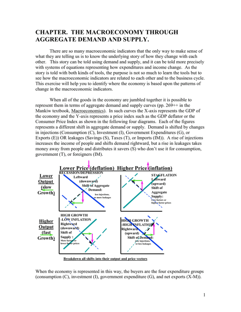
CHAPTER. THE MACROECONOMY THROUGH
AGGREGATE DEMAND AND SUPPLY.
There are so many macroeconomic indicators that the only way to make sense of
what they are telling us is to know the underlying story of how they change with each
other. This story can be told using demand and supply, and it can be told more precisely
with systems of equations representing how expenditures and income change. As the
story is told with both kinds of tools, the purpose is not so much to learn the tools but to
see how the macroeconomic indicators are related to each other and to the business cycle.
This exercise will help you to identify where the economy is based upon the patterns of
change in the macroeconomic indicators.
When all of the goods in the economy are jumbled together it is possible to
represent them in terms of aggregate demand and supply curves (pp. 269++ in the
Mankiw textbook, Macroeconomics). In such curves the X-axis represents the GDP of
the economy and the Y-axis represents a price index such as the GDP deflator or the
Consumer Price Index as shown in the following four diagrams. Each of the figures
represents a different shift in aggregate demand or supply. Demand is shifted by changes
in injections (Consumption (C), Investment (I), Government Expenditures (G), or
Exports (E)) OR leakages (Savings (S), Taxes (T), or Imports (IM)). A rise of injections
increases the income of people and shifts demand rightward, but a rise in leakages takes
money away from people and distributes it savers (S) who don’t use it for consumption,
government (T), or foreigners (IM).
Lower Price (deflation) Higher Price (inflation)
Lower
Output
(slow
Growth)
RECESSION/DEPRESSION
Leftward
(downward)
Shift of Aggregate
Demand:
STAGFLATION
Leftward
(upward)
Shift of
Aggregate
Supply:
less injections,
or more leakages
Less factors or
higher factor prices
Higher
Output
(fast
Growth)
HIGH GROWTH
-LOW INFLATION
Rightward
(downward)
Shift of
Supply :
More factors or
lower factor prices
HIGH GROWTH
-HIGH INFLATION
Rightward
(upward)
Shift of Demand:
mor injections,
or less leakages
Breakdown all shifts into their output and price vectors
When the economy is represented in this way, the buyers are the four expenditure groups
(consumption (C), investment (I), government expenditure (G), and net exports (X-M)).
1
Any determinant of demand that affects these four expenditure groups causes the demand
curve to shift.
The Aggregate Supply curve measures the capacity of the economy to produce
different levels of GDP. We are going to assume that we are looking at only one year
and that the economy has the flexibility to produce more GDP at higher prices. While
many economists believe that the aggregate supply curve is essentially vertical in the
long run (so that the capacity of the economy is not very responsive to higher prices), we
can assume here that some additional capacity can be made available if prices are high
enough. Aggregate supply is shifted by changes in factor availability or factor price
changes. Following are the four major factors and their factor prices:
FACTOR
Labor
Land
Capital
Entrepreneurship
FACTOR PRICE
Wages, salaries
“Rent”
Interest
Profit
While greater availability of a factor definitely shifts aggregate supply rightward, lower
factor prices are not unequivocal in their effect on supply. It depends upon the way in
which the factors of production respond to higher prices. For example if workers work
less when they receive higher pay (as in the case of a backward bending supply curve),
then the aggregate supply curve could actually shift leftward in response to higher wages.
Furthermore, higher wages could cause businesses to hire fewer people. On the other
hand, if more people are willing to work when wages rise, then aggregate supply could
actually shift to the right…. It depends on the circumstances.
EXAMPLE: Read the following excerpts from WSJ.com, entitled “China's Stimulus
Spurs U.S. Business” By JAMES T. AREDDY and TIMOTHY AEPPEL April 29,
2009
China's efforts to quickly pump up its economy are providing a muchneeded boost for U.S. businesses as well.
NOTE: In just this short beginning sentence, we can see that the Chinese government has
increased government expenditures (G), which because that is more of an injection, will
push aggregate demand to the right in china. But, because the resulting higher income
increases Chinese imports (IM), there will also be a shift leftward of the Chinese
aggregate demand curve because imports are a leakage to China. According to this
sentence, there is increased demand for U.S. exports, which means more of an injection
to the U.S. and therefore an aggregate demand shift to the right for the U.S. The article
continues:
Caterpillar Inc. Chief Executive James W. Owens says the company's
excavator sales in China have returned to record levels in recent months,
bouncing back from plummeting sales over the winter.
2
He says China continues to have a great need for infrastructure and that
projects there could start much more quickly than could similar projects
in the U.S. "It's something like nine months [in the U.S.] versus nine
weeks" in China, he says….
As a result, China, the world's third largest economy behind the U.S. and
Japan, may be the first major economy to recover.
"The hope is that China would become an engine of growth to drive the
global economy out of this severe recession -- much as the U.S. was the
engine of growth that drove the global economy after the dot-com
collapse," says Daniel Meckstroth, an economist at the Manufacturers
Alliance/MAPI, a public-policy group in Arlington, Va.
NOTE: Even though the excavator market is only a small fraction of total aggregate
demand, the first paragraph suggests that aggregate demand has shifted leftward in the
U.S., although the article isn’t giving us a reason. However, the second paragraph
indicates China is investing in “infrastructure.” Infrastructure is capital. That means that
the long run supply curve will shift to the right as the projects are completed. The second
paragraph also provides an interesting insight about why the Chinese market provides
such a stimulus to the U.S.; it moves faster. The multiplier works much more quickly
and therefore is larger during a shorter time period than in the U.S. The third paragraph
suggests the consequence; the multiplier will allow China to recover from the recession
more quickly than other nations. The fourth paragraph suggests that China is replacing
the U.S. in that role. The article continues:
Before the recession took root in the U.S. and then spread around the
world, companies talked about the powerful Chinese economy, which
was driving up demand and prices for a wide range of goods, from iron
ore to tractor tires.
Here we see evidence that factor prices were being driven up by Chinese demand. In the
U.S. the higher factor prices would shift the aggregate supply curve to the left, causing
higher prices in the U.S. As is the case with so many articles about an interdependent
world, there are likely to be many shifts of aggregate demand and supply reported in any
given article. The key skill is to be able to isolate each one and then it may be possible to
deduce the overall effect.
The four shifts in aggregate demand and supply, if large enough, produce the
effects shown in the above figure: stagflation (Price above normal and GDP below
normal), depression/recession (Price and GDP falling below normal), high growth(GDP
up) - high inflation (Price up above normal), and high growth (GDP up) -low inflation
(Price down or below normal). These shifts tend to occur in a cyclic pattern.
3
Let’s see what happens to the economy when consumers suddenly become
optimistic about the economy and start spending more money. They might finance this
consumption by going into debt in their credit cards. While the increased debt does not
affect aggregate demand or supply, the increased consumption shifts the demand curve to
the right as shown in Figure 1. However, the initial shift does not become immediately
visible to businesses or the government. Instead inventories begin to disappear a little
faster than usual at the current prices. If businesses don’t recognize this change in
inventory very quickly and leave prices unchanged, shortages will begin to develop, lines
will form, and people will resell the product to those who are willing to pay more- very
much like scalpers do with tickets at sports events. Even if businesses do recognize this
change in inventory quickly there may be lags in how quickly they can hire more workers
and expand capacity to increase production. The recognition lag and slowness in
responding means that orders are beginning to be stacked up and backlogged.
Companies are beginning to increase capacity utilization to fill their orders so that
customers will continue to be loyal.
FIGURE 1. RIGHTWARD SHIFT OF AGGREGATE DEMAND
CPI
index
Aggregate
Demand
Greater
Price
(inflation)
Greater
quantity
Aggregate
Supply
Disposable Income (Y)
The first chapter of the story of the business cycle is a sudden change across the
economy of the disequilibrium measures as shown in the following summary:
Upside of the Cycle
Change in inventories
Change in orders
Change in capacity utilization
Direction of indicator
+
+
For each of our disequilibrium indicators we are interested in the change of the indicator,
not the level of the indicator. Good media summaries about the economy should not only
4
compare the level of these indicators with previous periods, but should compare the
change in these indicators to past trends of change in the indicators.
As capacity utilization reaches to 100% and inventories fall toward zero, markets
will see higher prices as indicated in Figure 1. Even if manufacturers do not raise the
prices the middlemen will. Wholesalers and retailers who are close to the customer will
see the surge in aggregate demand and will recognize the opportunities available in the
market place to charge higher prices and they will charge the higher prices. By doing so,
they are rationing the product. Some people will no longer vie for goods and services at
the higher prices while those who are willing to pay the higher prices will receive the
goods and services. The Bureau of Labor Statistics in its monthly surveys of retailers
will discover and record the higher prices in the Consumer Price Index. The media will
report with lags of one to two months the percentage change in the Index and should
record a percentage change that is higher than past trends. Their articles will lament the
increase in the inflation rate, which is measured by the percentage change in the
Consumer Price Index.
The Consumer Price Index automatically triggers rises in social security payments
and cost-of-living adjustment (COLA) clauses in contracts- although it may take a year
for these changes to occur. Labor unions will look at rises in the cost of living and will
use them to negotiate higher wages in their contracts. These wage increases will take as
much three to five years to be reflected (depending upon how frequently a contract is
renegotiated). However, in the much larger non-unionized sector of the economy, wages
will also rise. The demand for labor is derived from the demand for the goods and
services that they produce. When demand in the product market shifts, the demand in the
labor market shifts in the same direction. The illustration of the higher demand for labor
would appear exactly as in Figure 1, except that the X-axis would be labor and the Y-axis
would be wages.
A much faster adjustment to higher inflation rates can occur in interest rates.
When businesses recognize that aggregate demand is rising for their goods, they suddenly
want to expand their businesses. Often the fastest way to undertake the necessary
additional gross investment is to borrow from the bank. Banks notice the increased
demand for money. Since the price of borrowing is the interest rate, the increased
demand for money leads to a rise in the interest rate. The illustration of the higher
demand for money would appear exactly as in Figure 1, except that the X-axis would be
money and the Y-axis would be interest rates.
Exchange can moderate the impacts of the business cycle. If inflation is
worsening with higher prices, wages, and interest rates a strengthening dollar actually
permits people to import goods which can ease any shortages that might be occurring at
home. Furthermore, since goods and services abroad are cheaper when a domestic
currency strengthens, there is a moderating influence on inflation; domestic businesses
can’t raise their prices too far without losing markets to foreign producers. However, if
an economy is running large trade deficits due to the economy’s growth, then the
exchange rate may fall in value. In this case foreign markets don’t provide as much of a
5
moderating influence. In fact interest rates may have to rise higher to offset the falling
value of the currency so that foreign investors won’t lose money by investing in the
United States.
Upside of the Cycle
Inflation (percentage change in prices)
Change in wages
Change in interest rates
Change in value of domestic currency
Direction of indicator
+
+
+
-
The National Accounts would now reflect the effects of the business cycle, but
preparing and reporting the information takes time and the media will be reporting the
changes in the economy months after those changes have occurred. It takes up to two
years before the final revisions of the data may be available on the national accounts. So
it may be possible only to guess where the economy is based upon disequilibrium and
price measures. Nevertheless, once we have an educated guess about how much
disposable income is changing it is possible to predict what is happening to the rest of the
items in the accounts. Figure 2 shows how the injections and leakages of the economy
are related to disposable income.
FIGURE 2
BEHAVIORAL RESPONSE OF EXPENDITURES TO INCOME
Imports
Taxes
Federal
Surplus
Federal
Deficit
Saving
Unintended
Inventory
Increase
Trade
Deficit
Investment
Exports
Government
Expenditures
D. Income
Trade
Surplus
D. Income
Unintended
Inventory
Decrease
D. Income
In the first diagram of Figure 2, government expenditures are examined with
respect to changes in disposable income (on the X-axis). With higher income the
diagram shows:

Taxes should be rising, particularly income taxes
6


Government expenditures may even fall because there are less social services
needed because there are fewer people unemployed or on welfare.
Since the federal deficit is the difference between government taxes and
government expenditures, the deficit decreases or even becomes a surplus as
income rises.
While the president of the United States often receives the blame for deficits and
surpluses, the state of the economy may be much more important, particularly in the first
two years of administration. However, historically some presidents have been able to
make a substantial change in expenditures or taxes in their first years, as did Franklin
Roosevelt, Ronald Reagan, and, most recently, George Bush in his tax rebate. In these
cases, the government expenditure and tax curves actually shift and change the income
level at which a deficit turns into a federal surplus. By the way, it’s not just the federal
government that works this way. Most of the state and local governments are thrown into
serious deficits when an economy goes into recession which forces serious and sudden
expenditure cutbacks if their laws require them to balance the budget every year.
In the second diagram of Figure 2, exports and imports are examined with respect
to changes in disposable income (on the X-axis). With higher income the diagram
shows:

Imports should be rising, as people buy more foreign imports.

Exports don’t change with domestic income, although they would shift with
foreign income which would affect how much foreigners would buy of
American goods. But only domestic income is shown on the X-axis.

Since the balance of trade (which is the same thing as net exports) is the
difference between exports and imports, the trade surplus decreases or
becomes a deficit as income rises.
While the president of the United States often receives the blame for deficits and
surpluses, the state of the economy may be much more important, particularly in the first
two years of administration. However, historically some presidents have been able to
make a substantial change in expenditures or taxes in their first years, as did Franklin
Roosevelt, Ronald Reagan, and, most recently, George Bush in his tax rebate. In these
cases, the government expenditure and tax curves actually shift and change the income
level at which a deficit turns into a federal surplus. By the way, it’s not just the federal
government that works this way. Most of the state and local governments are thrown into
serious deficits when an economy goes into recession which forces serious and sudden
expenditure cutbacks if their laws require them to balance the budget every year.
Since injections (Investment(I) + Government Expenditures(G) + Exports (X))
in the economy must equal the leakages (Savings (S) + Taxes (T) + Imports (IMP)) from
the economy, the following identity must hold:
I + G + X = S + T +IMP
But we can write this equation in terms of the fundamental balances:
7
Federal Deficit (G – T) + Trade Surplus ( X-IMP) = S – I
Savings and investment serve a balancing role. As shown in the last diagram of Figure 2,
there is an equilibrium disposable income level at which savings and investment perfectly
balance. But if disposable income falls below this equilibrium, savings will be below
investment and inventories will quickly drop below desirable levels. When inventories
drop below desired levels, economists say there is “involuntary disinvestment” or
“involuntary declines in inventory” in the economy. To avoid such disinvestments,
businesses will try to produce more output and increase their capacity to produce more
output. In effect they are increasing investment which will stimulate the economy to
grow. This increase in investment will further shift aggregate demand as shown in Figure
1.
As disposable income grows, consumption will also grow. Consumption (C) is
very closely related to income (Y). Figure 3 shows this relationship over the last thirty
years.
FIGURE 3. CONSUMPTION AND INCOME
When this relationship is shown logarithmically (lower diagram), the relationship
between the two is clearly constant. Notice how different our conclusions are about the
growth rate of the economy with the two diagrams in Figure 3. The logarithmic
presentation of the data clearly shows the slowing down of the economy while the raw
8
data (upper diagram) suggests that growth is accelerating. The behavior relationship
between disposable income (Y) and personal consumption (C) is so close it is commonly
represented as the following consumption function:
C= a + b* Y
The “a” refers to “autonomous consumption.” That is the component of consumption
that is not sensitive to income. In other words, no matter how low income might be, there
is a certain level of consumption that people will have. The “b” coefficient is referred to
as the “marginal propensity to consume (MPC)”. The marginal propensity to consume
shows how much of each extra dollar that is earned will be spent on consumption, rather
than saving. In other words people, have a choice to spend their income for consumption
today or consumption in the future (saving). The marginal propensity to save is simply
1-MPC.
We have now found several simultaneous indicators which are relied upon to
verify where we are in the business cycle. Each of these indicators is dependent upon
income:
Upside of the Cycle
Income, Output, Expenditure measures
Government Deficit
Trade surplus
Consumption, Saving
Imports
Taxes
Direction of indicator
+
+
+
+
+
+
There are many lagging indicators of the economy. Perhaps the most important of
these is unemployment and other measures of human resource utilization. When
businesses see inventories falling too quickly and the opportunity to sell more of their
output, they would like to hire more workers. But they may not be very certain that the
economy really is expanding. So they will first attempt to meet the greater needs for
workers by paying more overtime to their workers and expanding the number of average
hours worked by employees. In this way they can avoid hiring new workers who might
prove expensive to train and to let go if growth should fizzle. However, this expedient
can rapidly create morale problems and higher wage demands. Within months of a
growth surge in the economy, businesses will begin serious new hiring. Unfortunately
finding the right people may take a long time. It may be six months to several years
before companies are able to hire enough people to meet the new growth needs
adequately. The labor sector of the economy typically lags the economy.
Upside of the Cycle
Change in Average hours worked per week
Change in overtime hours
Direction of indicator
+
+
9
Changes in unemployment rate
Changes in employment
+
+
Many indicators serve a dual role of both reflecting and regulating the economy.
Prices are by far the most important example of such indicators. We have seen that an
upsurge of prices can reflect an upsurge in aggregate demand and the growth phase of a
business cycle. By looking at what is happening to prices, we can see where the
economy has been. However, they also have a regulating impact on the economy. As
the prices, wages, and interest rates rise, they begin to shut down the economy. As wages
catch up to an initial surge in price increases, profit margins are squeezed, possibly even
worse than if prices had never risen at all. As buyers close their pocket books to more
increases, businesses go bankrupt. The economy may enter a period of stagflation where
inflation is growing but the growth rate is falling and unemployment is becoming worse.
Prices are working like a thermostat to shut the economy down. Prices, wages, and
interest rates therefore reflect where the economy has been, but also where it is going.
Rising prices mean the economy for the last couple of months has likely been growing,
but accelerating price increases is likely to indicate that the economy within the next year
or two is likely to be experience slower and possibly negative growth rates.
There are many indicators of the economy such as the stock market, money
supply, government debt, private debt, etc. which have not been covered. Many of them
will be covered in later chapters. However, it is much more important for you to develop
your own indicators for barometric forecasting. Most published data are not reported
quickly enough to indicate the changes that are occurring to the economy. We can get
much better information by simply watching the environment around us. Here are some
of the items that are particularly useful to look for:
(1)
Gasoline Prices. Pick one service station that you pass every day and simply
observe the price of gasoline. Whenever the economy is booming transportation services
are being used by everyone and the increased demand of all goods and services is
anticipated by the oil industry in light of fixed supplies of oil and is therefore an early
warning of what is happening to the economy. Many industries like the auto and airplane
industries are likely to be doing as well oil because they are complementary goods to oil.
(2)
Housing Sales. As you become familiar with a neighborhood, you will begin to
get a sense of how long it takes for houses to move. If “for sale” signs are up for a long
time or there are relatively few houses being sold, it may mean that the real estate market
is slowing down. If you watch find out the prices of the houses that sell, you may be able
to judge how fast housing prices are rising which helps to understand inflation rates as
well as to indicate rising incomes of people. A strong housing market pulls the rest of the
economy along including the construction industry, construction materials, furniture,
gardening items, and a wide range of services.
(3)
Malls. If you regularly frequent a mall you may be able to judge when a mall is
experiencing above normal or below normal traffic in the stores. You may also see
evidence such as vacant store fronts or larger than normal sales that indicate economic
troubles. Malls provide a particularly broad summary of economic activity of the
economy.
10
(4)
Advertising in the Media. Events like the superbowl and NASCAR races are
extremely expensive advertising opportunities. Changes in who is buying the top
advertising spots or who is sponsoring major events may indicate important changes in
what industries are doing well in the economy. At the other extreme the want ads
sections of the newspaper provides insights into the tightness of the job market, the health
of the used goods sectors of the market, and the overall amount of economic activity.
(5)
New Construction Activity. Coming into a city for a trip can often indicate the
health of the city as well as the health of the economy. Busy construction cranes, newly
cleared land, full parking lots, shuttered buildings, dilapidated store fronts, maintenance
levels of streets, cleanliness of sidewalks, and a wide number of other visual clues can
provide information about how an economy is faring.
These are only a few ideas of what is easily available on a daily basis to give you clues
about the economy. You may find your own indicators that are much more useful to you
as early warnings of what may be happening to the economy.
THIS CHAPTER COULD HAVE BEEN WRITTEN IN REVERSE,
ILLUSTRATING THE CONCEPTS WITH A LEFTWARD SHIFT OF
AGGREGATE DEMAND. FOLLOWING IS ONE STUDENT’S EFFORT TO
REVERSE EVERYTHING. The Yellow marks are the words that must be changed
to do this successfully.
CHAPTER. THE MACROECONOMY THROUGH
AGGREGATE DEMAND AND SUPPLY.
There are so many macroeconomic indicators that the only way to make sense of
what they are telling us is to know the underlying story of how they change with each
other. This story can be told using demand and supply, and it can be told more precisely
with systems of equations representing how expenditures and income change. As the
story is told with both kinds of tools, the purpose is not so much to learn the tools but to
see how the macroeconomic indicators are related to each other and to the business cycle.
This exercise will help you to identify where the economy is based upon the patterns of
change in the macroeconomic indicators.
The economy can be represented with by one aggregate demand curve and one
aggregate supply curve. When all of the goods in the economy are jumbled together in
this way, the X-axis represents the GDP of the economy and the Y-axis represents a price
index such as the GDP deflator or the Consumer Price Index. When the economy is
represented in this way, the buyers are the four expenditure groups (consumption (C),
investment (I), government expenditure (G), and net exports (X-M)). Any determinant of
demand that affects these four expenditure groups causes the demand curve to shift.
The Aggregate Supply curve measures the capacity of the economy to produce
different levels of GDP. We are going to assume that we are looking at only one year
and that the economy has the flexibility to produce more GDP at higher prices. While
many economists believe that the aggregate supply curve is essentially vertical in the
long run (so that the capacity of the economy is not very responsive to higher prices), we
11
can assume here that some additional capacity can be made available if prices are high
enough.
Let’s see what happens to the economy when consumers suddenly become
pessimistic about the economy and start spending less money. They might finance this
consumption by going into debt in their credit cards. While the increased debt does not
affect aggregate demand or supply, the decreased consumption shifts the demand curve to
the left as shown in Figure 1. However, the initial shift does not become immediately
visible to businesses or the government. Instead inventories begin to increase a little
faster than usual at the current prices. If businesses don’t recognize this change in
inventory very quickly and leave prices unchanged, surpluses will begin to develop, lines
will disappear, and people will resell the product to those who are willing to pay morevery much like scalpers do with tickets at sports events. Even if businesses do recognize
this change in inventory quickly there may be lags in how quickly they can get rid of
workers and decrease capacity to decrease production. The recognition lag and slowness
in responding means that inventory is beginning to be stacked up and backlogged.
Companies are beginning to decrease capacity utilization to sell off their inventory so that
customers will continue to be loyal.
FIGURE 1. LEFTWARD SHIFT OF AGGREGATE DEMAND
CPI
index
Aggregate
Demand
Lower
Price
(deflation)
Aggregate
Supply
Smaller
quantity
Disposable Income (Y)
The first chapter of the story of the business cycle is a sudden change across the
economy of the disequilibrium measures as shown in the following summary:
Downside of the Cycle
Change in inventories
Change in orders
Direction of indicator
+
12
Change in capacity utilization
-
For each of our disequilibrium indicators we are interested in the change of the indicator,
not the level of the indicator. Good media summaries about the economy should not only
compare the level of these indicators with previous periods, but should compare the
change in these indicators to past trends of change in the indicators.
As capacity utilization approaches 0% and inventories increase, markets will see
lower prices as indicated in Figure 1. Even if manufacturers do not lower the prices the
middlemen will. Wholesalers and retailers who are close to the customer will see the
decrease in aggregate demand and will recognize the need in the market place to charge
lower prices and they will charge the lower prices. By doing so, they are getting rid of
the product. Some people will now no longer vie for goods and services at the lower
prices, while those who are willing to pay the higher prices will receive the goods and
services. The Bureau of Labor Statistics in its monthly surveys of retailers will discover
and record the lower prices in the Consumer Price Index. The media will report with lags
of one to two months the percentage change in the Index and should record a percentage
change that is lower than past trends. Their articles will lament the decrease in the
inflation rate, which is measured by the percentage change in the Consumer Price Index.
The Consumer Price Index automatically triggers falls in social security payments
and cost-of-living adjustment (COLA) clauses in contracts- although it may take a year
for these changes to occur. Labor unions will look at falls in the cost of living and will
use them to negotiate lower wages in their contracts. These wage decreases will take as
much three to five years to be reflected (depending upon how frequently a contract is
renegotiated). However, in the much larger non-unionized sector of the economy, wages
will also fall. The demand for labor is derived from the demand for the goods and
services that they produce. When demand in the product market shifts, the demand in the
labor market shifts in the same direction. The illustration of the lower demand for labor
would appear exactly as in Figure 1, except that the X-axis would be labor and the Y-axis
would be wages.
A much faster adjustment to lower inflation rates can occur in interest rates.
When businesses recognize that aggregate demand is falling for their goods, they
suddenly want to downsize their businesses. Often the fastest way to undertake the
necessary adjustments is to stop borrowing from the bank. Banks notice the decreased
demand for money. Since the price of borrowing is the interest rate, the decreased
demand for money leads to a fall in the interest rate. The illustration of the lower demand
for money would appear exactly as in Figure 1, except that the X-axis would be money
and the Y-axis would be interest rates.
Exchange can moderate the impacts of the business cycle. If deflation is
worsening with lower prices, wages, and interest rates, a weakening dollar actually
prevents people from importing goods which can ease any surpluses that might be
occurring at home. Furthermore, since goods and services abroad are more expensive
when a domestic currency weakens, there is a moderating influence on deflation;
13
domestic businesses don’t have to worry about losing markets to foreign producers.
However, if an economy is running large trade surplus due to the economy’s downfall,
then the exchange rate may increase in value. In this case foreign markets don’t provide
as much of a moderating influence. In fact interest rates may have to fall lower to offset
the rising value of the currency so that foreign investors won’t lose money by investing in
the United States.
Downside of the Cycle
Inflation (percentage change in prices)
Change in wages
Change in interest rates
Change in value of domestic currency
Direction of indicator
+
The National Accounts would now reflect the effects of the business cycle, but
preparing and reporting the information takes time and the media will be reporting the
changes in the economy months after those changes have occurred. It takes up to two
years before the final revisions of the data may be available on the national accounts. So
it may be possible only to guess where the economy is based upon disequilibrium and
price measures. Nevertheless, once we have an educated guess about how much
disposable income is changing it is possible to predict what is happening to the rest of the
items in the accounts. Figure 2 shows how the injections and leakages of the economy
are related to disposable income.
FIGURE 2
BEHAVIORAL RESPONSE OF EXPENDITURES TO INCOME
Imports
Taxes
Federal
Surplus
Federal
Deficit
Saving
Unintended
Inventory
Increase
Trade
Deficit
Investment
Exports
Government
Expenditures
D. Income
Trade
Surplus
D. Income
Unintended
Inventory
Decrease
D. Income
14
In the first diagram of Figure 2, government expenditures are examined with
respect to changes in disposable income (on the X-axis). With lower income the diagram
shows:

Taxes should be falling, particularly income taxes

Government expenditures may even rise because there are more social
services needed because there are more people unemployed or on welfare.

Since the federal deficit is the difference between government taxes and
government expenditures, the deficit increases or even becomes a surplus as
income falls.
While the president of the United States often receives the blame for deficits and
surpluses, the state of the economy may be much more important, particularly in the first
two years of administration. However, historically some presidents have been able to
make a substantial change in expenditures or taxes in their first years, as did Franklin
Roosevelt, Ronald Reagan, and, most recently, George Bush in his tax rebate. In these
cases, the government expenditure and tax curves actually shift and change the income
level at which a deficit turns into a federal surplus. By the way, it’s not just the federal
government that works this way. Most of the state and local governments are thrown into
serious deficits when an economy goes into recession which forces serious and sudden
expenditure cutbacks if their laws require them to balance the budget every year.
In the second diagram of Figure 2, exports and imports are examined with respect
to changes in disposable income (on the X-axis). With lower income the diagram shows:

Imports should be falling, as people buy less foreign imports.

Exports don’t change with domestic income, although they would shift with
foreign income which would affect how much foreigners would buy of
American goods. But only domestic income is shown on the X-axis.

Since the balance of trade (which is the same thing as net exports) is the
difference between exports and imports, the trade deficit increases or becomes
a deficit as income falls.
While the president of the United States often receives the blame for deficits and
surpluses, the state of the economy may be much more important, particularly in the first
two years of administration. However, historically some presidents have been able to
make a substantial change in expenditures or taxes in their first years, as did Franklin
Roosevelt, Ronald Reagan, and, most recently, George Bush in his tax rebate. In these
cases, the government expenditure and tax curves actually shift and change the income
level at which a deficit turns into a federal surplus. By the way, it’s not just the federal
government that works this way. Most of the state and local governments are thrown into
serious deficits when an economy goes into recession which forces serious and sudden
expenditure cutbacks if their laws require them to balance the budget every year.
Since injections (Investment(I) + Government Expenditures(G) + Exports (X))
in the economy must equal the leakages (Savings (S) + Taxes (T) + Imports (IMP)) from
the economy, the following identity must hold:
15
I + G + X = S + T +IMP
But we can write this equation in terms of the fundamental balances:
Federal Deficit (G – T) + Trade Surplus ( X-IMP) = S – I
Savings and investment serve a balancing role. As shown in the last diagram of Figure 2,
there is an equilibrium disposable income level at which savings and investment perfectly
balance. But if disposable income falls below this equilibrium, savings will be below
investment and inventories will quickly drop below desirable levels. When inventories
drop below desired levels, economists say there is “involuntary disinvestment” or
“involuntary declines in inventory” in the economy. To avoid such disinvestments,
businesses will try to produce more output and increase their capacity to produce more
output. In effect they are increasing investment which will stimulate the economy to
grow. This increase in investment will further shift aggregate demand as shown in Figure
1.
As disposable income grows, consumption will also grow. Consumption (C) is
very closely related to income (Y). Figure 3 shows this relationship over the last thirty
years.
FIGURE 3. CONSUMPTION AND INCOME
16
When this relationship is shown logarithmically (lower diagram), the relationship
between the two is clearly constant. Notice how different our conclusions are about the
growth rate of the economy with the two diagrams in Figure 3. The logarithmic
presentation of the data clearly shows the slowing down of the economy while the raw
data (upper diagram) suggests that growth is accelerating. The behavior relationship
between disposable income (Y) and personal consumption (C) is so close it is commonly
represented as the following consumption function:
C= a + b* Y
The “a” refers to “autonomous consumption.” That is the component of consumption
that is not sensitive to income. In other words, no matter how low income might be, there
is a certain level of consumption that people will have. The “b” coefficient is referred to
as the “marginal propensity to consume (MPC)”. The marginal propensity to consume
shows how much of each extra dollar that is earned will be spent on consumption, rather
than saving. In other words people, have a choice to spend their income for consumption
today or consumption in the future (saving). The marginal propensity to save is simply
1-MPC.
We have now found several simultaneous indicators which are relied upon to
verify where we are in the business cycle. Each of these indicators is dependent upon
income:
Upside of the Cycle
Income, Output, Expenditure measures
Government Deficit
Trade surplus
Consumption, Saving
Imports
Taxes
Direction of indicator
+
+
+
+
+
+
There are many lagging indicators of the economy. Perhaps the most important of
these is unemployment and other measures of human resource utilization. When
businesses see inventories falling too quickly and the opportunity to sell more of their
output, they would like to hire more workers. But they may not be very certain that the
economy really is expanding. So they will first attempt to meet the greater needs for
workers by paying more overtime to their workers and expanding the number of average
hours worked by employees. In this way they can avoid hiring new workers who might
prove expensive to train and to let go if growth should fizzle. However, this expedient
can rapidly create morale problems and higher wage demands. Within months of a
growth surge in the economy, businesses will begin serious new hiring. Unfortunately
finding the right people may take a long time. It may be six months to several years
before companies are able to hire enough people to meet the new growth needs
adequately. The labor sector of the economy typically lags the economy.
17
Upside of the Cycle
Change in Average hours worked per week
Change in overtime hours
Changes in unemployment rate
Changes in employment
Direction of indicator
+
+
+
+
Many indicators serve a dual role of both reflecting and regulating the economy.
Prices are by far the most important example of such indicators. We have seen that an
upsurge of prices can reflect an upsurge in aggregate demand and the growth phase of a
business cycle. By looking at what is happening to prices, we can see where the
economy has been. However, they also have a regulating impact on the economy. As
the prices, wages, and interest rates rise, they begin to shut down the economy. As wages
catch up to an initial surge in price increases, profit margins are squeezed, possibly even
worse than if prices had never risen at all. As buyers close their pocket books to more
increases, businesses go bankrupt. The economy may enter a period of stagflation where
inflation is growing but the growth rate is falling and unemployment is becoming worse.
Prices are working like a thermostat to shut the economy down. Prices, wages, and
interest rates therefore reflect where the economy has been, but also where it is going.
Rising prices mean the economy for the last couple of months has likely been growing,
but accelerating price increases is likely to indicate that the economy within the next year
or two is likely to be experience slower and possibly negative growth rates.
There are many indicators of the economy such as the stock market, money
supply, government debt, private debt, etc. which have not been covered. Many of them
will be covered in later chapters. However, it is much more important for you to develop
your own indicators for barometric forecasting. Most published data are not reported
quickly enough to indicate the changes that are occurring to the economy. We can get
much better information by simply watching the environment around us. Here are some
of the items that are particularly useful to look for:
(1)
Gasoline Prices. Pick one service station that you pass every day and simply
observe the price of gasoline. Whenever the economy is booming transportation services
are being used by everyone and the increased demand of all goods and services is
anticipated by the oil industry in light of fixed supplies of oil and is therefore an early
warning of what is happening to the economy. Many industries like the auto and airplane
industries are likely to be doing as well oil because they are complementary goods to oil.
(2)
Housing Sales. As you become familiar with a neighborhood, you will begin to
get a sense of how long it takes for houses to move. If “for sale” signs are up for a long
time or there are relatively few houses being sold, it may mean that the real estate market
is slowing down. If you watch find out the prices of the houses that sell, you may be able
to judge how fast housing prices are rising which helps to understand inflation rates as
well as to indicate rising incomes of people. A strong housing market pulls the rest of the
economy along including the construction industry, construction materials, furniture,
gardening items, and a wide range of services.
(3)
Malls. If you regularly frequent a mall you may be able to judge when a mall is
experiencing above normal or below normal traffic in the stores. You may also see
18
evidence such as vacant store fronts or larger than normal sales that indicate economic
troubles. Malls provide a particularly broad summary of economic activity of the
economy.
(4)
Advertising in the Media. Events like the superbowl and NASCAR races are
extremely expensive advertising opportunities. Changes in who is buying the top
advertising spots or who is sponsoring major events may indicate important changes in
what industries are doing well in the economy. At the other extreme the want ads
sections of the newspaper provides insights into the tightness of the job market, the health
of the used goods sectors of the market, and the overall amount of economic activity.
(5)
New Construction Activity. Coming into a city for a trip can often indicate the
health of the city as well as the health of the economy. Busy construction cranes, newly
cleared land, full parking lots, shuttered buildings, dilapidated store fronts, maintenance
levels of streets, cleanliness of sidewalks, and a wide number of other visual clues can
provide information about how an economy is faring.
These are only a few ideas of what is easily available on a daily basis to give you clues
about the economy. You may find your own indicators that are much more useful to you
as early warnings of what may be happening to the economy.
© copyright
19