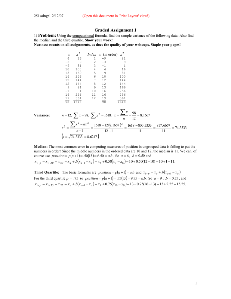
251solngr1 2/12/07
(Open this document in 'Print Layout' view!)
Graded Assignment 1
1) Problem: Using the computational formula, find the sample variance of the following data: Also find
the median and the third quartile. Show your work!
Neatness counts on all assignments, as does the quality of your writeups. Staple your pages!
x2
x
4
-3
-9
10
13
16
12
12
9
-1
16
19
98
Variance:
16
9
81
100
169
256
144
144
81
1
256
361
1618

x

n  12,
s 
1
2
3
4
5
6
7
8
9
10
11
12
x  98,
2
s2
Index x (in order) x 2
 nx
n 1

2
-9
-3
-1
4
9
10
12
12
13
16
16
19
98
81
9
1
16
81
100
144
144
169
256
256
361
1618
x 2  1618 , x 
 x  98  8.1667
n
12
1618  12 8.1667 
1618  800 .3333 817 .6667


 74.3333
12  1
11
11
2

74 .3333  8.6217

Median: The most common error in computing measures of position in ungrouped data is failing to put the
numbers in order! Since the middle numbers in the ordered data are 10 and 12, the median is 11. We can, of
course use position  pn  1  .5013  6.50  a.b . So a  6 , .b  0.50 and
x1 p  x1.50  x.50  xa  .bxa1  xa   x6  0.50x7  x6   10  0.50(12 10)  10  1  11.
Third Quartile: The basic formulas are position  pn  1  a.b and x1 p  x a  .bx a 1  x a 
For the third quartile p  .75 so position  pn  1  .7513  9.75  a.b . So a  9 , .b  0.75 , and
x1 p  x1.75  x.25  xa  .bxa1  xa   x9  0.75x10  x9   13  0.75(16 13)  13  2.25  15.25.
1
251solngr1 2/12/07
(Open this document in 'Print Layout' view!)
2) Computer Assignment
To get credit for the remainder of this assignment you must turn in original spreadsheets.
This Computer Assignment has as its goal to do most of Problem G3 using Excel.
Step 1: Open up an Excel worksheet and start by filling locations A1-14 by labeling the column with: the
word "Class" in A1, the labels for the classes in A2 to A13, the word "Total" in A14. If you have trouble
with some of these labels, using single quotes can help.
Step 2: Put the abbreviation "Mdpt" for midpoint in B1. Fill Column B with the midpoints for the classes by
putting 2.5 in B2 and 7.5 in B3. Highlight B2 and B3 and drag the fill handle down to fill the cells down to
B13. (To do this point to the highlighted area until you get a black cross, then move the pointer down.) You
should now have the numbers 2.5 to 57.5 in column B.
Step 3: You now need the frequency column. Put "f " in C1. Copy the frequencies in C2 through C13.
Highlight cell C14 and find the AutoSum logo, which is simply a summation sign
on the top. Click
 
on the summation sign and "enter." This will give you the sum of the frequencies. Remember that
f n.

Step 4: Now compute the cumulative frequencies in column C. Head the column with "F" and copy the one
from C2 to D2. In D3 put "=D2+C3." In D4 put "=D3+C4." Now highlight D3 and D4 and use the fill
handle to fill in D5 through D13. The last cumulative frequency in D13 should be 90.
Step 5: Label column E with "xf " or "fx." To compute this column, put "=B2*C2" in E2 and "=B3*C3" in
E3. Use the fill handle to fill in the rest of the products down to E13. Use the AutoSum feature to put a total
fx in E14.
 
Step 6: In column F you will compute x 2 f or fx2 . Label the column "xsqf " or "fxsq." Now F2 will be
done with "=B2*E2," and F3 with "=B3*E3" and you can fill the column down to F13 with the fill handle,
fx 2 using AutoSum.
and get its sum
 
Step 7: Now compute the mean, variance and standard deviation using the computational formulas. In K1
put the words "n =" and copy n into L1, perhaps by writing "=c14" in L1. In K2 put the words "Mean =,"

fx
fx 2  nx 2
2
and in L2 compute x 
by using "=E14/C14." Now you are ready to do s 
. Put
n 1
n
fx 2 is in F14, n is in C14 and x is in L2. You should compute x 2 by
"Var =" in K3. Remember that



multiplying the mean by itself, so the formula in L3 should be "=(F14-C14*L2*L2)/(C14-1)." You should
get 132.5843.
Now you need the standard deviation, which is simply the square root of the variance, so put "StDev =" in
K4 and "=SQRT(L3)" in L4.
2
251solngr1 2/12/07
(Open this document in 'Print Layout' view!)
Step 8: Now we are going to use the definitional formula to compute the skewness. Start by writing the
value that you got for the mean in cell M2. Do not copy this value or use an equation to get it into M2, just
type it in. Excel will mess up some calculations if you do. Use the fill handle to fill the M column with the
mean.
You are now going to compute x  x  , f x  x  , f x  x 2 and f x  x 3 in columns G, H, I and J. Head
these columns with "x' ," "'fx'," "fx'sq" and "fx'cu." In G2 enter "=B2-M2" and use the fill handle to put the
values of the midpoints minus the mean in G2 through G13. In H2 enter "=G2*C2, " use the fill handle to
fill in to H13 and use AutoSum to put the sum of column H in H14. This sum should be zero. In I2 enter
"=G2*H2" and use the fill handle again. In I14 get
 f x  x 
2
. You can use this to check the accuracy of
your variance computation. In J2 enter "=G2*I2" and again fill the column. Use AutoSum to get
n
f x  x 3 by
f x  x 3 in J14. Then in cell K5 type "K3 =," and in L5 compute k 3 
n  1n  2
typing "=C14*J14/((C14-1)*(c14-2))


Step 9: Use the formatting toolbar to center the first row of columns B through J. Make any other formatting
changes that you think would improve the legibility if the spreadsheet and print out the results.
a) For the original solution to this problem see SolnG3A.
b) For the Excel solution see grdat1 . You have to have Excel to read this.
3) Research Assignment. Talk to about 20 students. Ask them how many hours they studied over
some period of time - it could be a day, several days or a week. Use Excel to analyze your data. Put a
heading in cell A1 and your data below it. Use the "Tools" pull-down menu. Pick "Data Analysis" and
"Descriptive Statistics." Check "Labels in First Row." and "Summary Statistics." (If you cannot find this,
use Tools and Add-Ins to put in the analysis packs.) Specify a range (like A1: A50) Comment on the output
in a short paragraph. Are you close to the mean? Why or why not. The skewness statistic computed here is
K3, so compute a measure of relative skewness and tell me if the data is highly skewed and in what
direction. Write in brief literate English!
Possible Solution: As an example, your data in column A might be something like:
Times, 1, 2, 2, 3, 4, 4, 4, 5, 5, 5, 7, 8, 8, 8, 9, 10, 11, 12, 14, 16,
16, 16
The data analysis software gave me the results below on the 4th page of
my worksheet.
Column1
Mean 7.727272727
Standard Error
1.017555466
Median
7.5
Mode 4
Standard Deviation
4.772758194
Sample Variance
22.77922078
Kurtosis
-0.851661267
Skewness
0.515444345
Range 15
Minimum
1
Maximum
16
Sum
170
Count 22
3
251solngr1 2/12/07
(Open this document in 'Print Layout' view!)
And I might have said:
The data above represent the weekly study time of 22 randomly
selected respondents. I study 30 hours a week, so that my study time
seems to be far above any of the times in my survey. The skewness
coefficient of 0.515 when divided by the third power of the standard
deviation, gives me a relative skewness of about 0.005, which indicates
that the data is almost symmetrical (actually barely skewed to the
right). This seems to be brought out by the similarity of the median and
the mean, even though the mode is much smaller.
An actual copy of more recent results, set up so that the data and
results are on the same page appears below.
Times
1
2
2
3
4
4
4
5
5
5
7
8
8
8
9
10
11
12
14
16
16
16
Times
Mean
Standard
Error
Median
Mode
Standard
Deviation
Sample
Variance
Kurtosis
Skewness
Range
Minimum
Maximum
Sum
Count
7.727273
1.017555
7.5
4
4.772758
22.77922
-0.85166
0.515444
15
1
16
170
22
4
251solngr1 2/12/07
(Open this document in 'Print Layout' view!)
4) Extra Credit
a) The data was set up as follows in columns c1, c2 and c10:
Row
f
x
Class
1
2
3
4
5
6
7
8
9
10
11
12
1
0
3
7
15
16
12
11
9
9
6
1
2.5
7.5
12.5
17.5
22.5
27.5
32.5
37.5
42.5
47.5
52.5
57.5
0-4.9
5-9.9
10-14.9
15-19.9
20-24.9
25-29.9
30-34.9
35-39.9
40-44.9
45.49.9
50-54.9
55-59.9
These were saved in the Minitab data file 251G3o. The three command files were run by copying from the
website, with the following results. This is a highly edited version of my 2003 run. The 2005 run got
identical results, but had to be done anyway because of changes in Minitab. Some blank lines have been
edited out to preserve continuity. # creates instructions that are not read by Minitab and is used for student
names, routine names and comments .
—————
9/4/2003 6:57:31 PM
————————————————————
Welcome to Minitab, press F1 for help.
MTB > Retrieve "C:\Documents and Settings\RBOVE.WCUPANET\My
Documents\Drive D\MINITAB\251G3o.MTW".
Retrieving worksheet from file: C:\Documents and
Settings\RBOVE.WCUPANET\My Documents\Drive D\MINITAB\251G3o.MTW
# Worksheet was saved on Thu Sep 04 2003
MTB > #Roger Bove
MTB > #grp.mtb
Here’s where I copied in the first subroutine
from the website.
Results for: 251G3o.MTW
MTB >
MTB >
here.
MTB >
MTB >
MTB >
MTB >
MTB >
MTB >
MTB >
MTB >
MTB >
MTB >
MTB >
MTB >
MTB >
MTB >
MTB >
let c3 = c1*c2
let c4 = c3*c2
#You have already given these columns names
#They will be designated by column numbers
let c5 = c4*c2
name k1 'n'
#The Built-in constants k1-k9 are given names.
name k2 'mean'
name k3 'Sfx'
name k4 'Sfx2'
name k5 'Sfx3'
name k7 'Sfx^'
name k8 'Sfx^2'
name k9 'Sfx^3'
let k1 = sum(c1)
#This is how we sum a column.
let k3 = sum(c3)
let k4 = sum(c4)
let k5 = sum(c5)
let k2 = k3/k1
print c10, c1-c5
5
251solngr1 2/12/07
(Open this document in 'Print Layout' view!)
Data Display - These are the columns on the first page of the solution to problem G3.
Row
1
2
3
4
5
6
7
8
9
10
11
12
Class
0-4.9
5-9.9
10-14.9
15-19.9
20-24.9
25-29.9
30-34.9
35-39.9
40-44.9
45.49.9
50-54.9
55-59.9
f
1
0
3
7
15
16
12
11
9
9
6
1
x
2.5
7.5
12.5
17.5
22.5
27.5
32.5
37.5
42.5
47.5
52.5
57.5
fx
2.5
0.0
37.5
122.5
337.5
440.0
390.0
412.5
382.5
427.5
315.0
57.5
fxsq
6.3
0.0
468.8
2143.8
7593.8
12100.0
12675.0
15468.8
16256.3
20306.3
16537.5
3306.3
fxcu
16
0
5859
37516
170859
332750
411938
580078
690891
964547
868219
190109
MTB > print k1-k5
Data Display
n
90.0000
#This is k1.
mean
32.5000
#This is k2.
Sfx
2925.00
#This is k3.
Sfx2
106863
#This is k4.
Sfx3
MTB >
MTB >
MTB >
MTB >
MTB >
MTB >
MTB >
4252781
let c6 = c2-k2
let c7 = c1*c6
let c8 = c7*c6
let c9 = c8*c6
let k7 = sum(c7)
let k8 = sum(c8)
let k9 = sum(c9)
#This is k5.
 f  n  90 


 x   fx  2925 .0  32 .5 


n
90
 fx  2925 .0
 fx  106862 .5
 fx  4252781 .250 


2
3
6
251solngr1 2/12/07
(Open this document in 'Print Layout' view!)
MTB > print c10, c6-c9
Data Display
These are the columns on the Third page of the solution to problem G3.
Row
Class
x^
1
2
3
4
5
6
7
8
9
10
11
12
0-4.9
5-9.9
10-14.9
15-19.9
20-24.9
25-29.9
30-34.9
35-39.9
40-44.9
45.49.9
50-54.9
55-59.9
-30
-25
-20
-15
-10
-5
0
5
10
15
20
25
fx^
-30
0
-60
-105
-150
-80
0
55
90
135
120
25
fx^sq
fx^cu
900
0
1200
1575
1500
400
0
275
900
2025
2400
625
-27000
0
-24000
-23625
-15000
-2000
0
1375
9000
30375
48000
15625
MTB > print k7-k9
Data Display
Sfx^
0
#This is k7.
Sfx^2
11800.0
#This is k8.
Sfx^3
12750.0
MTB > end
MTB > #grpv.mtb
#This is k9.
MTB
MTB
MTB
MTB
>
>
>
>
let k6 =
name k10
name k11
name k17
k1-1
'var1'
'var2'
'stdev'
#In k10
s12
MTB > let k11 = k1*k2*k2
MTB > let k11 = k4-k11
#k11 s 22 
MTB > let k11 = k11/k6
>
>
>
>
>
>
name k14 'k31'
name k16 'k32'
name k18 'g11'
name k19 'g12'
let k12 = k6-1
let k13 = k1/k6
MTB > let k13 = k13/k12
3
 f x  x 

n 1
 fx
2
 nx 2
n 1

2

11800
 132 .584
89
106862 .50  90 32 .52
 132 .584
89
# In k12 s  variance  132.584  11.515
MTB > let k17 = sqrt(k11)
MTB > end
MTB
MTB
MTB
MTB
MTB
MTB
2
Here’s where I copied in the second subroutine
from the website.
#k6 is n  1 .
#The Built-in constants are given names.
MTB > let k10 = k8/k6
MTB > #grps.mtb
 f x  x   0
 f x  x   11800
 f x  x   12750
Here’s where I copied in the third subroutine
from the website.
#The 3rd k-statistic or skewness
#Relative skewness.
#
n2
# In k13
n
(n  1)( n  2)
7
251solngr1 2/12/07
(Open this document in 'Print Layout' view!)
n
(n  1)( n  2)
# k 31
MTB > let k14 = k13*k9
 f x  x 
3
MTB > let k15 = 2*k1*k2*k2*k2
MTB > let k16 = 3*k2*k4
MTB > let k15 = k5-k16+k15
n
(n  1)( n  2)
# In k16 k 32 
MTB > let k16 = k13*k15
90
12750   146 .514
89 88 

 fx
3
 3x
 fx
2
 2nx 3

MTB > let k18 = k16/k11
# g 11 
MTB > let k18 = k18/k17
k 32
s
3

146 .514

 132 .584 
3
146 .514
 0.094 (Got twisted.)
1526 .640
MTB > let k19 = k14/k11
# In k19 g 12 
MTB > let k19 = k19/k17
k 31
s

3
146 .514
 132 .584 
3

146 .514
 0.094
1526 .640
MTB > print k1-k19
Data Display
n
90.0000
mean
32.5000
Sfx
2925.00
Sfx2
106863
Sfx3
4252781
K6
89.0000
Sfx^
0
Sfx^2
11800.0
Sfx^3
12750.0
# n 1
 f x  x 
2

11800
 132 .584
89

106862 .50  90 32 .52
 132 .584
89
var1
132.584
# s12 
var2
132.584
# s 22 
K12
88.0000
# n2
K13
0.0114913
#
k31
146.514
# k 31
K15
12750.0
#
k32
146.514
# k 32 
stdev
11.5145
g11
0.0959714
g12
0.0959714
# s  variance  132.584  11.515
k
146 .514
146 .514
# g 11  32


 0.094
3
3
1526 .640
s
132 .584
k
146 .514
146 .514
# g 12  31


 0.094
3
3
1526
.640
s
132 .584
MTB > end
n 1
 fx
2
 nx 2
n 1
n
Intermediate computation.
(n  1)( n  2)
 f x  x   89 88 12750   146 .514
 3 x  fx  2nx  Intermediate.
n
(n  1)( n  2)
 fx
3
3
2
n
(n  1)( n  2)
90
3
 fx




3
 3x
 fx
2
 2nx 3

#This is the end of what you were asked to do.
8