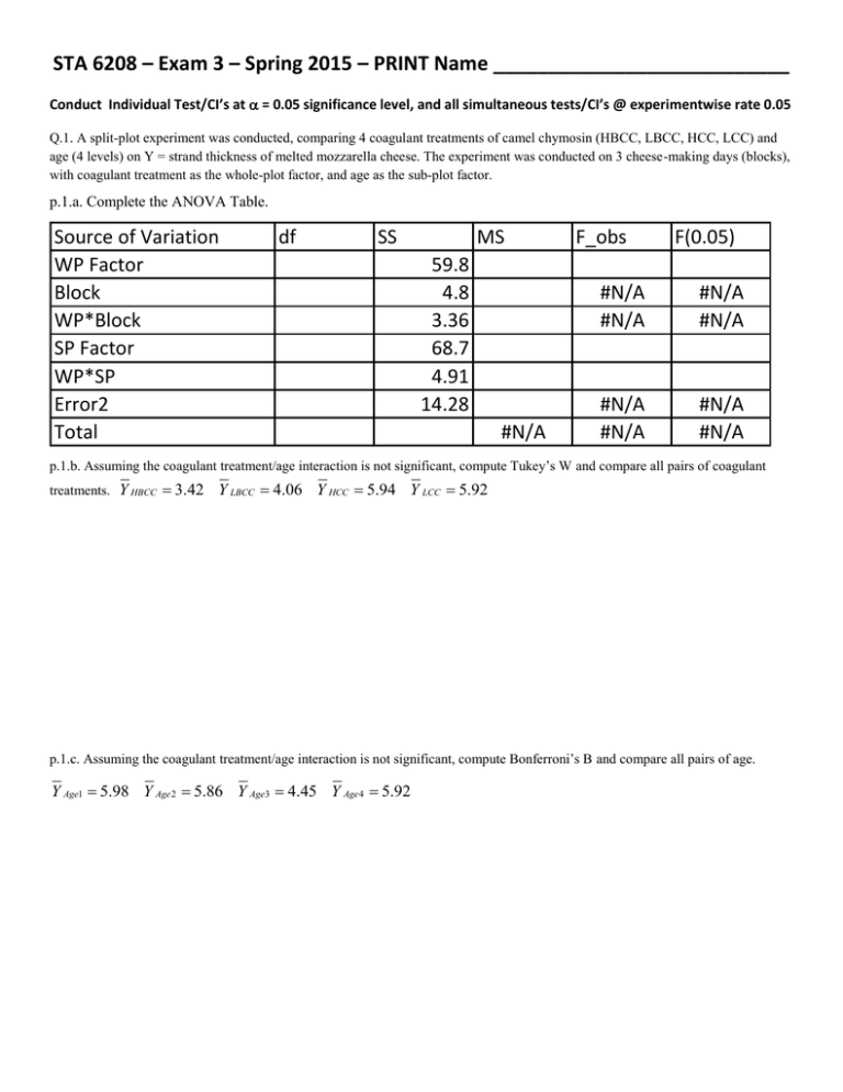
STA 6208 – Exam 3 – Spring 2015 – PRINT Name ___________________________
Conduct Individual Test/CI’s at  = 0.05 significance level, and all simultaneous tests/CI’s @ experimentwise rate 0.05
Q.1. A split-plot experiment was conducted, comparing 4 coagulant treatments of camel chymosin (HBCC, LBCC, HCC, LCC) and
age (4 levels) on Y = strand thickness of melted mozzarella cheese. The experiment was conducted on 3 cheese-making days (blocks),
with coagulant treatment as the whole-plot factor, and age as the sub-plot factor.
p.1.a. Complete the ANOVA Table.
Source of Variation
WP Factor
Block
WP*Block
SP Factor
WP*SP
Error2
Total
df
SS
MS
59.8
4.8
3.36
68.7
4.91
14.28
#N/A
F_obs
F(0.05)
#N/A
#N/A
#N/A
#N/A
#N/A
#N/A
#N/A
#N/A
p.1.b. Assuming the coagulant treatment/age interaction is not significant, compute Tukey’s W and compare all pairs of coagulant
treatments. Y HBCC  3.42
Y LBCC  4.06 Y HCC  5.94 Y LCC  5.92
p.1.c. Assuming the coagulant treatment/age interaction is not significant, compute Bonferroni’s B and compare all pairs of age.
Y Age1  5.98 Y Age 2  5.86 Y Age3  4.45 Y Age 4  5.92
Q.2. A study compared doses of a drug on female rats’ activity levels in a maze. A sample of 91 rats were selected, and randomized
such that 21 rats received the Control Dose, 25 received Low Dose, 24 received Medium Dose, and 21 received High Dose. Each rat’s
activity levels were observed at 4 time points after dosing (15, 30, 45, and 60 minutes).
Hint: There are a total of 21+25+24+21=91 rats in the study.
Complete the following ANOVA table. The dose and time means are given in the second table.
Source
Dose
Rat(Dose)
Time
Dose*Time
Error2
Total
df
SS
MS
176677
F
F(0.05)
Significant?
#N/A
#N/A
#N/A
#N/A
#N/A
#N/A
#N/A
#N/A
#N/A
2161
465319
#N/A
Trt
n_dose Time1
Time2
Time3
Time4
Mean
Control
21
165.9
136.3
121.4
103.4
131.8
LowDose
25
167.8
148.4
123.7
118.4
139.6
MidDose
24
168.3
140.3
117.2
109.8
133.9
HighDose
21
184.4
156.2
136.3
122.7
149.9
Sum/Mean
91
171.3
145.3
124.4
113.7
138.7
Q.3. A bioavailability study for sulpride involved 3 treatments (sulpride alone (A), sulpride with sucralafate (B), and
sulpride with antacid (C)). It was conducted in 3 time periods with 6 subjects in a replicated latin square. The ANOVA
and the design are given below, for Y = Urinary excretion of sulpride in 24 hours. The means are:
Y A  31.0 Y B  18.6 Y C  20.9 Y   23.5
p.3.a. Complete the ANOVA table.
Source
Trts
Periods
Subjects
Error
Total
df
SS
MS
51
380
1083
#N/A
F_obs
#N/A
#N/A
#N/A
#N/A
F(0.05)
#N/A
#N/A
#N/A
#N/A
Subject\Period
1
2
3
4
5
6
1
A
C
B
C
B
A
2
B
A
C
A
C
B
3
C
B
A
B
A
C
p.3.b. How many times does each treatment appear in each subject?
p.3.b. How many times does each treatment appear in each Period?
p.3.c. Use Tukey’s HSD to compare all pairs of treatment means.
HSDij = _______________________________
Connect trts that are not significantly different B C
A
Q.4. A randomized complete block design is conducted with t (fixed) treatment in r blocks.
Case 1: Random Blocks
yij     i  b j  eij
i  1,..., t ; j  1,..., b
t

i 1
i
 0 b j ~ NID  0,  b2  eij ~ NID  0,  2 
p.4.a. E(yij) =
p.1.b. V(yij) =
p.4.c.(i≠i’) COV(yij , yi’j) =
p.1.d. (j≠j’) COV(yij , yij’) =
p.4.e. Derive
 



V y i , COV y i , y i ' , V y i  y i '

(SHOW ALL WORK)
b   e 
j
ij
Case 2: Fixed Blocks
yij     i   j  eij
i  1,..., t; j  1,..., r
t
 i  0
i 1
p.4.f. E(yij) =

j 1
j

 0 eij ~ NID 0,  2

p.1.g. V(yij) =
p.4.h. (i≠i’) COV(yij , yi’j) =
p.4.j. Derive V
r
 y ,
i

p.1.i. (j≠j’) COV(yij , yij’) =


COV y i , y i ' , V y i  y i '

(SHOW ALL WORK)
Q.5.