Hidden Markov Random Field and FRAME
modelling for TCA image analysis
Katy Streso and Francesco Lagona
StatLab, Office of Statistics and Information Services, Max Planck Institute for
Demographic Research, Konrad - Zuse - Strasse 1, 18057 Rostock, Germany
streso@demogr.mpg.de and lagona@demogr.mpg.de
Summary. Tooth Cementum Annulation (TCA) is an age estimation method carried out on thin cross sections of the root of the human tooth. Age is computed by
adding the tooth eruption age to the count of annual incremental lines which are
called tooth rings and appear in the cementum band. Algorithms to denoise and
segment the digital image of the tooth section are considered a crucial step towards
computer-assisted TCA. The approach in this paper relies on modelling the images
as hidden Markov random fields, where gray values are assumed to be pixelwise
conditionally independent and normally distributed, given a hidden random field of
labels. These unknown labels have to be estimated to segment the image. To account for long-range dependence among the observed values and for periodicity in
the placement of tooth rings, the Gibbsian label distribution is specified by a potential function that incorporates macro-features of the TCA image (a FRAME model).
An estimation of the model parameters is made by an EM algorithm exploiting the
mean field approximation of the label distribution. Segmentation is based on the
predictive distribution of the labels given the observed gray values.
Key words: EM, FRAME, Gibbs distribution, (hidden) Markov random field,
mean field approximation, TCA
1 Introduction
Tooth Cementum Annulation [WGV03] is an age estimation method based on annual
incremental appositions in the cementum of mammalian teeth. A 90-110 µm thick
cross section, polished or unpolished, is photographed using a Leica DC350F camera
system with bright-field and 200 or 400 times magnification. TCA images are then
8 or 16 bit gray scale pictures of 1030x1300 or 1016x1300 pixels in size. The dark
parts of the annual lines, often called tooth rings, are empirically 1 to 3 µm thick
and roughly result in thin lines of 5 to 20 pixel with 400 times magnification.
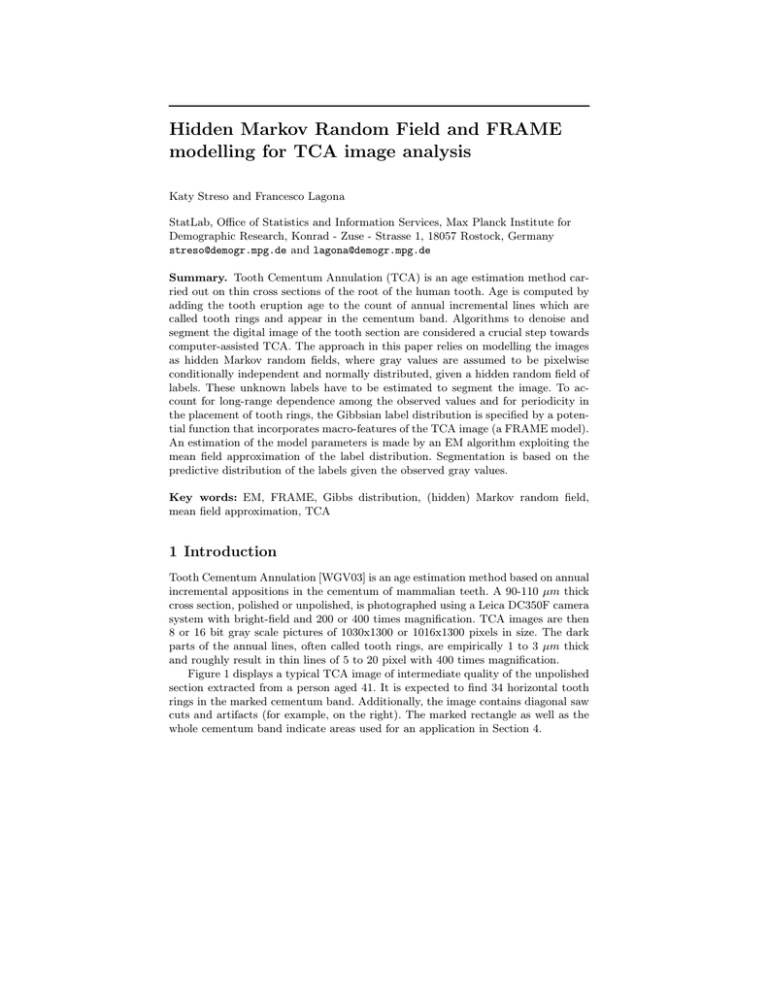
Figure 1 displays a typical TCA image of intermediate quality of the unpolished
section extracted from a person aged 41. It is expected to find 34 horizontal tooth
rings in the marked cementum band. Additionally, the image contains diagonal saw
cuts and artifacts (for example, on the right). The marked rectangle as well as the
whole cementum band indicate areas used for an application in Section 4.
Katy Streso and Francesco Lagona
cementum band
1226
Fig. 1. An unpolished TCA image (IS-0000666 from the TCA database of the MPI)
Paleodemographers at the Max Planck Institute for Demographic Research use
large databases of images as depicted in Figure 1 to identify mortality profiles of
past human populations. Computer-aided evaluation of TCA images is considered
an important step towards defining a protocol for TCA-based age estimation.
In the course of this paper, TCA images are denoised and segmented by a Hidden
Markov Random Field (HMRF) model, were the distribution of the hidden field is
specified by a FRAME prior [ZWM97]. This is a Markov Random Field (MRF) that
models macro-features of TCA images such as long-range auto-correlation among
observed gray values and periodic placement of tooth rings. The HMRF is introduced
Section 2. Section 3 describes the estimation of the model via an EM algorithm that
exploits the mean field approximation of the hidden field distribution. In Section
4 we specify the FRAME model for the application to TCA images and present
sensible results of fitting the hidden FRAME model to TCA images.
Hidden MRF and FRAME modelling for TCA image analysis
1227
2 The Hidden FRAME Model
HMRF modelling allows us to address both denoising and segmentation by means
of a labelling problem [Li01]. To illustrate, let S = {1, . . . , N M } be the set of pixels
forming a rectangular lattice of size N × M . In the course of this paper, a pixel will
interchangeably be denoted by i, or (x, y) when the two dimensions of the lattice
need to be emphasized. The observed image is represented by array Y , where Yi ∈ R
is the gray value observed at pixel i. Value Yi is assumed to be drawn from the ith
continuous random variable Yi , belonging to the random field Y = (Y1 , . . . , YNM ).
Analogously, we define array λ of labels λi ∈ G = {0, 1, . . . , G} that need to be
estimated at each pixel and assume that λi is sampled from the discrete random
variable Λi , defined as the ith coordinate of the random field Λ = (Λ1 , . . . , ΛNM ).
In the HMRF setting, the joint distribution of Y is modelled according to the
mixture
f (Y ) =
X
P (λ)
λ∈G N ×M
Y
i∈S
f (Yi |λi ) ,
(1)
with known number of components, where P (λ) is the distribution of a Markov
random field and f (Y |λ) is called cost function. The choice of both depends on the
application. For TCA images, we have chosen a Gaussian cost function
−
1
f (Yi |λi , θ) = √
e
2πσλi
(Yi −µλi )2
2σ2
λi
,
where parameters θ = {µg , σg2 |g ∈ G} are unknown. MRF P (λ) may model spatial
dependencies by means of specifying a neighborhood structure. More precisely, let
us define
• a neighboring relationship as a binary relationship on lattice S that is antireflexive and symmetric;
• neighborhood N (i) of pixel i as the set N (i) = {j ∈ S|j neighbor of i} and
• neighborhood system N as the set of all neighborhoods N = {N (i)|i ∈ S}.
Under this setting, random field Λ is a MRF with respect to neighborhood system
N , if for all λ ∈ G N×M
1. P (λ) > 0 (positivity),
2. P λi |λS\i = P (λi |λN(i) ) (Markovianity).
The specific form of the MRF model that will be utilized for TCA images is called
FRAME, which stands for Filters, Random Fields and Maximum Entropy and was
mainly developed in [ZWM97], [ZWM98] and [ZM97]. In the FRAME model, prior
knowledge of images is efficiently modelled by convolving label image λ with suitable
filters and by evaluating the filter responses. In its simplest version, the FRAME
distribution is a Gibbs distribution
P (λ) =
1
e
Z
P
i∈S
φ[(FT ∗λ)(i)]
,
(2)
where Z is the normalizing constant. The energy function involves one filter FT that
is known up to parameter T . The filter responses (FT ∗ λ)(i) to λ at pixels i are
1228
Katy Streso and Francesco Lagona
evaluated pixelwise by the potential function φ. The choice of the parametric family FT and function φ is driven by the application (Section 4). The hidden FRAME
model thus elegantly combines two important areas of texture analysis: HMRF modelling and filtering theory, and it can be applied to a wide variety of even large scale
textures.
3 Parameter Estimation and Segmentation
In order to estimate θ and T , the maximum likelihood estimates (MLE) θ̂ and T̂ can
in principle be found by maximizing the likelihood function L(θ, T |Y ) as presented
in Equation (1). However, this maximization is intractable because of the size of
label space G N×M . The EM algorithm is a widely used technique to solve this kind
of problem. The algorithm depends on the predictive probability usually computed
via MCMC. In our application this is computationally too expensive because of the
size of neighborhoods and the size of images that are considered for TCA application.
We suggest to use mean field approximation (MFA) to make the EM tractable.
Let us recall that the EM algorithm starts with preliminary estimates θ (0) and
T (0) of the parameters θ and T , and then proceeds iteratively by alternating two
steps. In the E-step of the t-th iteration, the conditional expectation of the complete
log-likelihood, with respect to the unknown labels λ, say
h
i
E log P (Y, λ|θ, T )|Y, θ (t−1), T (t−1) =
Z
P λ|Y, θ (t−1), T (t−1) log P (λ, Y |θ, T )dλ
λ∈G N ×M
is calculated, where θ (t−1) and T (t−1) are the estimates from the previous iteration. The M-step of the EM algorithm maximizes this expectation to update θ
and T . Since each iteration is guaranteed to increase the (incomplete) log-likelihood
L(θ, T |Y ) under mild assumptions, the EM algorithm will converge to a local maximum [MK97]. With a Gaussian random field, the EM algorithm reduces to the three
updating formulas [MK97]
P
µ(t)
g =
Yi P λi = g|Yi , λN(i) , θ (t−1) , T (t−1)
i∈S
P
i∈S
σg(t)
2
=
P λi = g|Yi , λN(i) , θ (t−1) , T (t−1)
P
i∈S
(t)
Yi − µg
P
2
,
P λi = g|Yi , λN(i) , θ (t−1) , T (t−1)
P λi = g|Yi , λN(i) , θ (t−1) , T (t−1)
,
i∈S
G
XX
T (t) = argmax
log P λi = g|λN(i) , T P λi = g|Yi , λN(i) , θ (t−1), T (t−1)
{T }
i∈S g=0
(3)
The conditional probabilities P λi = g|Y, λN(i) , θ, T are not available in closed
form and could be evaluated by an MCMC algorithm [ZBS01]. This would require
to generate a Markov chain at each pixel, which is too time consuming for large scale
Hidden MRF and FRAME modelling for TCA image analysis
1229
textures modelled by large neighborhoods. The alternative approach we suggest is
based on the approximation
Y
P (λ) ≈
i∈S
P λi |λ̃N(i) .
(4)
In this paper, the configuration λ̃ is chosen according to the theory of mean field
approximation [CFP03], where λ̃ is set to the expected values of the label image:
λ̃j = E[λj ] for all j ∈ N (i). The parameter estimates can therefore be updated by
Equations (3) and replacing λN(i) therein by λ̃N(i) , which are computed iteratively.
Our EM algorithm then takes the following form:
EM algorithm using MFA for fitting a hidden FRAME model
1. input TCA image Y
2. initialize label configuration λ(0) by thresholding and initialize parameters
3. for t = 1 : tmax
4. hλi = λ(t−1) (update label image)
5. for each site i (randomly permuted)
6.
for g = 0 : G
7.
calculate the cond. prob. f Yi |λi = g, µ(t−1) , σ (t−1) according to Equ.
(??)
8.
approximate
P
e
G
P
φ
j∈N (i)
9.e
P
φ
j∈N (i)
F
T
the
prior
P λi = g|λN(i) , T (t−1)
prob.
≈
(t−1) ∗λ (j)
F
T (t−1)
∗λ (j)
calculate the posterior probability
g=0
P λi = g|Yi , λN(i) , θ
(t−1)
,T
(t−1)
=
G
P
g=0
G
P
g·P
λi =g|Yi ,λN (i) ,θ
P P λ
g=0
G
calculate the expected label hλi i =
set λ(t) = hλi
for g = 0 : G (update parameters)
13.
14.
update µg and σg
according to Equations (3)
update T according to Equation (3)
(t)
g=0
i =g|Yi ,λN (i) ,
(t−1)
,T (t−1)
θ (t−1) ,T (t−1)
2
The initialization of λ and the sequential updating of the labels were chosen
according to the recommendations in [CFP03]. The number of iterations tmax was
selected such that the absolute relative change in the log-likelihood
L(θ (t−1) , T (t−1) |Y ) =
X
i∈S
log
G
X
f Yi |λi = g, θ (t−1) P λi = g|λN(i) , T (t−1)
10.
11.
12.
f Yi |λi = g, θ (t−1) P λi = g|λN(i) , T (t−1)
P λi = g|Yi , λN(i) , θ (t−1) , T (t−1) .
(5)
g=0
−6
over the last five iterations
is less than 10
. Segmentation can finally be carried
out by exploiting P λi = g|Yi , λN(i) , θ̂, T̂ by means of thresholding.
1230
Katy Streso and Francesco Lagona
4 Application
This Section is devoted to specifying the ingredients of the FRAME model that we
have used for TCA image analysis: the filter family FT and the potential function
φ. A simulated image that was generated by the Gibbs sampler will illustrate this
model. Finally results from fitting a Gaussian hidden FRAME model to TCA images
are shown.
Filtering theory is well recognized in texture analysis at least since [JF91].
Marčelja [Ma80] has shown that two-dimensional Gabor functions closely conform
to the receptive field profiles of simple cells in the striate cortex. We define filters
FT,α on the basis of real valued, even-symmetric Gabor functions:
GcosT,α (x, y) = c · e
(
− rx′2 +y′2
2T 2
)
cos
2π ′
x ,
T
(6)
with x′ = x cos α + y sin α, y ′ = −x sin α + y cos α, r = 4 being the aspect ratio and c
being a normalizing factor. The Gaborcosine function above is an elongated Gaussian
bell, multiplied by a cosine wave, where parameter T changes the wavelength and
α determines the orientation of the cosine wave. For example, Figure 2 (a and b)
shows the Gaborcosine function for T = 16, α = 0 and x, y ∈ [−13, 13]. This filter
can capture waves or lines of width 16 and orientation 0◦ .
(a)
(b)
(c)
Fig. 2. 3-D surface (a) and image (b) of a Gaborcosine function with T = 16 and
α = 0, and a typical image of 128x128 pixels in size simulated by the Gibbs sampler
using the FRAME model (2) with this filter, φ = |.| and 8 gray levels (c).
In the application for TCA images, we fix α = 0, which is the main direction
of tooth rings. In order to cover the range of possible tooth ring widths, we chose
T ∈ {2, 4, 6, 8, 10, 12, 14, 16, 18}. We remark that our approach is different to that
in [ZWM97], because we are interested in reconstructing tooth rings that resemble
only one feature of interest. We do not want to synthesize perceptional equivalent
images, including noise. Besides simplifying the FRAME model to incorporate only
one filter (one feature), the potential function φ that evaluates the filter response
is assumed to be known and chosen to be the simplest among the upright curves,
namely the absolute value φ = |.|.
Hidden MRF and FRAME modelling for TCA image analysis
1231
Figure 2 (c) displays a typical image drawn from the FRAME model using the
Gaborcosine filter with parameters T = 16 and α = 0 and the absolute valued
potential function. This image comes very close to the ideal TCA image that one
could have in mind about parallel running tooth rings. The orientation and width of
these lines are determined by both parameters of the Gaborcosine filter. The image
in Figure 2 (c) was generated by single Gibbs sampling. (See [SL05].)
To uncover the black and white labelling (G = {0, 1}) of the TCA image in
Figure 1, a Gaussian hidden Markov random field was fitted. The MRF model was
specified by the FRAME model (2). Parameters µ0 , µ1 and a common variance σ 2
as well as the filter parameter T were estimated by an EM algorithm, as stated in
Section 2. Label image λ was obtained from the mean field at the last iteration.
Figure 3 (a) shows the predictive probability P (λi |λ̃N(i) , θ̂, T̂ ) of the pixels in the
cementum band of Figure 1 (including the artifact on the right), where θ̂ and T̂
are the estimates of the last iteration. The parameter estimates are the means µ̂0 =
29026, µ̂1 = 29052, the common variance σ̂ 2 = 4.8 · 107 , and the ring width T̂ = 14.
For illustration purposes, a smaller part (marked in Figures 1 and 3 (a)) of this
mean field is thresholded (λi = 0 if P (λi |λ̃N(i) , θ̂, T̂ ) < 0.5 and λi = 1 otherwise).
The middle lines of the black rings are then superimposed on the original image (see
Figure 3 (b)).
(a)
(b)
Fig. 3. The mean field approximation of the cementum band of TCA image 1 (a)
and its black rings overlayed onto part of the original (b)
The median number of dark rings in label image 3 (a) is 35. From the known age,
the expected number of tooth rings (the known age minus average tooth eruption
age) is 33.61 in the image presented in Figure 1.
Additional experiments with TCA images of mixed quality gave the following
results:
These results are competitive to the manually counted number of rings.
1232
Katy Streso and Francesco Lagona
Image number of rings Image number of rings Image number of rings
IS-000 expected estimated IS-000 exp. estim. IS-000 exp. estim.
0231
40.94
46
0688 35.44
34
1547 38.19
28
0592
60.39
64
1157 34.39
30
1692 34.39
34
35.44
33
1225 40.94
46
0682
5 Conclusion
TCA images can be efficiently modelled by a HMRF and were evaluated by the
estimation of the predictive label distribution, via an EM algorithm using MFA.
Despite of the good overall age estimate, visual inspection of Figure 3 shows two
drawbacks for TCA application: tooth rings are not well detected and bifurcations
occur in the label image. This is due to the rigidity of the hidden FRAME model that
uses one filter, and hereby accounts only for strong local changes of tooth rings. To
add flexibility one could model non-homogeneity by estimating location dependent
filters, or one could additionally estimate the filter orientation α. But estimating the
filter parameter T at each pixel gave unstable and biased results. Experiments for the
second approach as well as standard error calculations are in progress. Additionally
one should test mode field and simulated field approximation [CFP03] for quality
and speed instead of approximating (4) by mean field approximation.
References
[WGV03] Wittwer-Backofen, U., Gampe, J., Vaupel, J.W.: Tooth Cementum Annulation for Age Estimation: Results from a Large Known-Age Validation Study.
American Journal of Physical Anthropology, 123(2), 119–129 (2003)
[ZWM97] Zhu, S.C., Wu, Y.N., Mumford, D.B.: Minimax Entropy Principle and Its
Application to Texture Modeling. Neural Computation, 9(8), 1627–1660 (1997)
[Li01] Li, S.Z.: Markov Random Field Modeling in Image Analysis. Springer, Tokyo
[et al.] (2001)
[ZWM98] Zhu, S.C., Wu, Y., Mumford, D.B.: Filters, Random Fields and Maximum
Entropy (FRAME): Towards a Unified Theory for Texture Modeling. International Journal of Computer Vision Archive, 27(2), 107–126 (1998)
[ZM97] Zhu, S.C., Mumford, D.B.: Prior Learning and Gibbs Reaction-Diffusion.
IEEE Trans. PAMI, 19(11), 1236–1250 (1997)
[MK97] McLachlan, G.J., Krishnan, T.: The EM Algorithm and Extensions. John
Wiley & Sons, New York (1997)
[ZBS01] Zhang, Y., Brady, M., Smith, S.: Segmentation of Brain MR Images
Through a Hidden Markov Random Field Model and the ExpectationMaximization Algorithm. IEEE Trans. on Medical Imaging, 20(1), 45–57 (2001)
[CFP03] Celeux, G., Forbes, F., Peyrard, N.: EM procedures using mean field-like
approximations for Markov model-based image segmentation. Pattern Recognition, 36(1), 131–144 (2003)
[JF91] Jain, A.K., Farrokhnia, F.: Unsupervised Texture Segmentation Using Gabor
Filters. Pattern Recognition, 24(12), 1167–1186 (1991)
[Ma80] Marčelja, S.: Mathematical description of the responses of simple cortical
cells. Journal of the Optical Society of America, 70(11), 297–300 (1980)
Hidden MRF and FRAME modelling for TCA image analysis
1233
[SL05] Streso, K., Lagona, F.: Hidden Markov Random Field and FRAME Modelling for TCA Image Analysis. Proceedings of the Third IASTED International
Conference on Signal Processing, Pattern Recognition, and Applications, 310 –
315 (2006)