Proceedings of the Tenth International AAAI Conference on
Web and Social Media (ICWSM 2016)
Precise Localization of Homes and Activities:
Detecting Drinking-While-Tweeting Patterns in Communities
Nabil Hossain, Tianran Hu,
Roghayeh Feizi
Dept. Computer Science
University of Rochester
Rochester, New York
{nhossain,thu}@cs.rochester.edu
Ann Marie White
Jiebo Luo, Henry Kautz
Dept. Psychiatry
University of Rochester
School of Medicine & Dentistry
Rochester, New York
AnnMarie White@urmc.rochester.edu
Dept. Computer Science
University of Rochester
Rochester, New York
{jluo,kautz}@cs.rochester.edu
Abstract
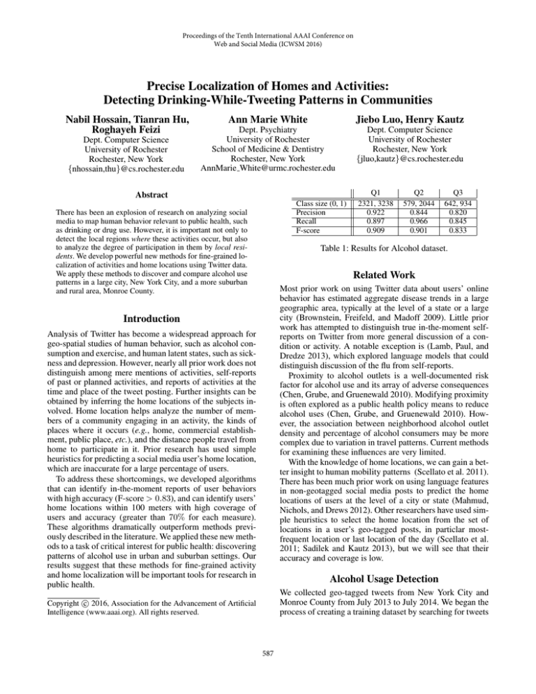
Class size (0, 1)
Precision
Recall
F-score
There has been an explosion of research on analyzing social
media to map human behavior relevant to public health, such
as drinking or drug use. However, it is important not only to
detect the local regions where these activities occur, but also
to analyze the degree of participation in them by local residents. We develop powerful new methods for fine-grained localization of activities and home locations using Twitter data.
We apply these methods to discover and compare alcohol use
patterns in a large city, New York City, and a more suburban
and rural area, Monroe County.
Q1
2321, 3238
0.922
0.897
0.909
Q2
579, 2044
0.844
0.966
0.901
Q3
642, 934
0.820
0.845
0.833
Table 1: Results for Alcohol dataset.
Related Work
Most prior work on using Twitter data about users’ online
behavior has estimated aggregate disease trends in a large
geographic area, typically at the level of a state or a large
city (Brownstein, Freifeld, and Madoff 2009). Little prior
work has attempted to distinguish true in-the-moment selfreports on Twitter from more general discussion of a condition or activity. A notable exception is (Lamb, Paul, and
Dredze 2013), which explored language models that could
distinguish discussion of the flu from self-reports.
Proximity to alcohol outlets is a well-documented risk
factor for alcohol use and its array of adverse consequences
(Chen, Grube, and Gruenewald 2010). Modifying proximity
is often explored as a public health policy means to reduce
alcohol uses (Chen, Grube, and Gruenewald 2010). However, the association between neighborhood alcohol outlet
density and percentage of alcohol consumers may be more
complex due to variation in travel patterns. Current methods
for examining these influences are very limited.
With the knowledge of home locations, we can gain a better insight to human mobility patterns (Scellato et al. 2011).
There has been much prior work on using language features
in non-geotagged social media posts to predict the home
locations of users at the level of a city or state (Mahmud,
Nichols, and Drews 2012). Other researchers have used simple heuristics to select the home location from the set of
locations in a user’s geo-tagged posts, in particlar mostfrequent location or last location of the day (Scellato et al.
2011; Sadilek and Kautz 2013), but we will see that their
accuracy and coverage is low.
Introduction
Analysis of Twitter has become a widespread approach for
geo-spatial studies of human behavior, such as alcohol consumption and exercise, and human latent states, such as sickness and depression. However, nearly all prior work does not
distinguish among mere mentions of activities, self-reports
of past or planned activities, and reports of activities at the
time and place of the tweet posting. Further insights can be
obtained by inferring the home locations of the subjects involved. Home location helps analyze the number of members of a community engaging in an activity, the kinds of
places where it occurs (e.g., home, commercial establishment, public place, etc.), and the distance people travel from
home to participate in it. Prior research has used simple
heuristics for predicting a social media user’s home location,
which are inaccurate for a large percentage of users.
To address these shortcomings, we developed algorithms
that can identify in-the-moment reports of user behaviors
with high accuracy (F-score > 0.83), and can identify users’
home locations within 100 meters with high coverage of
users and accuracy (greater than 70% for each measure).
These algorithms dramatically outperform methods previously described in the literature. We applied these new methods to a task of critical interest for public health: discovering
patterns of alcohol use in urban and suburban settings. Our
results suggest that these methods for fine-grained activity
and home localization will be important tools for research in
public health.
Alcohol Usage Detection
We collected geo-tagged tweets from New York City and
Monroe County from July 2013 to July 2014. We began the
process of creating a training dataset by searching for tweets
c 2016, Association for the Advancement of Artificial
Copyright Intelligence (www.aaai.org). All rights reserved.
587
Classifier
SVM-1
SVM-2
SVM-3
Negative features
club, shot, party, #turnup, yak, lean, crown, root beer,
root, wasted, turn up, turnup, binge, drunk in love,
in love, water, fucked up, fucked, water bottles
she, he, your, people, they, are, my mom,
drunk people, guy, #mention you, her, for me,
baby, their, his, see, most, talking, the drunk
hangover, need, want, was, when, or, real, alcoholic,
for, last night, will, wanna, tonight, got, weekend,
yesterday, was drunk
Positive features
drunk, beer, wine, alcohol, vodka, drink, tequila,
hangover, drinking, liquor, #beer, hammered,
take shot, get wasted, champagne, booze, ciroc, rum
will, when you, bad, when drunk, with, am,
get drunk, through, drink, dad, us, friday, more,
still, little, drinking, free, pong
#url, shot, here, #mention when, bottle of wine,
drank, now, think, one, good, vodka, by, me and, outside, hammered, haha, drive
Table 2: Top weighted features for alcohol classifiers (sorted in descending order of importance).
Positive Features
Check-in ratio
Margin between top two check-ins
PageRank Score
Last destination with inactive late night
Reversed PageRank score
Negative Features
Margin below next higher check-in
Margin under next higher PageRank
Margin under next higher Reversed PageRank
Rank of Reversed PageRank
Rank of PageRank
Weight
2.03
0.19
0.19
0.12
0.09
Weight
-0.30
-0.28
-0.21
-0.07
-0.07
Table 3: Top SVM features for home prediction.
example, the input for SVM-2 (SVM for question Q2) includes only the tweets labeled by SVM-1 as “yes” and answered by Turkers for Q2. This restricts the dataset distribution as we go down the hierarchy. Compared to a single flattened multi-class classifier, hierarchical classifiers are easier
to optimize, and, because they have a restricted feature set,
are less prone to overfitting. For each SVM, we used 80% of
the labeled data for training and the remaining 20% for testing. We applied 5 fold cross validation to reduce overfitting
and used the F-score for model selection.
The results in Table 1 show high precision and recall at
each stage, although each measure decreases as the classifier
goes down the hierarchy, most likely because there is less
training data at each stage. As shown in Table 2, SVM-1 uses
features related to alcoholic drinks to determine whether the
tweet is related to drinking alcoholic beverages. SVM-2 distinguishes self-reports from general drinking discussion by
using pronouns and implicit references to drinking. SVM3 identifies drinking-in-the-moment by using temporal features (e.g., “last night”, “now”) and features related to the
urge to drink (e.g., “need”, “want”).
Figure 1: Flowchart for latent activity detection.
that included a drinking-related keyword (e.g., “drunk”,
“beer”, “party”). Amazon Mechanical Turk workers then answered three yes/no questions for each tweet:
Q1: Does the tweet make any reference to drinking alcoholic beverages?
Q2: if so, is the tweet about the tweeter him or herself
drinking alcoholic beverages?
Q3: if so, is it likely that the tweet was sent at the time and
place the tweeter was drinking alcoholic beverages?
Finally, we reduced lexical variation by replacing all mentions by the term #mention, web addresses by the term #url,
and sequences of three or more of the same letter to two
letters (e.g., “YESSSS” becomes “YESS”). We call a tweet
that is “yes” for question Q3 a “user-drinking-now” tweet.
From training data1 , we created separate trigram linguistic
feature sets for each question. To reduce overfitting, we only
kept the top N most-frequent features, where N = 25% of
the size of the training set size for the corresponding question. For each question, we trained a linear support vector
machine (SVM) to predict the answer. As shown in Figure 1,
these SVMs are hierarchical (Koller and Sahami 1997). For
1
Home Location Prediction
We collected geo-tagged tweets sent from the greater New
York City (July 2012) and the Bay area (Jun-Aug 2013).
Each tweet was assigned to a cell in 100x100 meter grid.
We call a tweet from a location (grid cell) a “check-in”. We
considered users who had sent at least 5 geo-tagged tweets,
and computed their hourly traces. If a user appeared in several different locations in an hour, we used the location with
the highest number of check-ins. If a user did not tweet during an hour, the location for that hour was set to “unknown”.
available in: cs.rochester.edu/u/nhossain/icwsm-16-data.zip
588
0.8
●
●
●
●
SVM
Most check−in
PageRank
Re−PageRank
Total geo-tagged tweets
Passed keyword filter
Passed SVM-1
Passed SVM-2
Passed SVM-3
Correlation with outlet density
●
Monroe
1,537,979
26,858
13,108
12,178
8,854
0.237
●
0.4
Applicable scope
0.6
●
NYC
1,931,662
51,321
24,258
23,110
18,890
0.390
Table 4: Classification of drinking-related tweets on NYC
and Monroe datasets.
●
●
●
0.2
●
●
●
Figure 2 shows how our methods compare with three
other single-feature based methods suggested in the literature in terms of accuracy and coverage. At every accuracy
level, our method covers more users. When we set the accuracy of each method to 70%, our classifier obtains 71%
coverage for NY City. No previous work achieves anywhere
near this coverage, accuracy, or localization resolution.
●
0.0
●
0.60
0.65
0.70
0.75
0.80
0.85
0.90
Accuracy
Figure 2: Comparison of our SVM method for home location
prediction to prior approaches in New York City dataset, as
coverage and accuracy vary.
Analysis of Alcohol Consumption via Twitter
We applied our methods to data from New York City
and from Monroe County. As shown in Table 4, for each
drinking-related question, NYC has a higher proportion of
tweets marked positive compared to the corresponding proportion in Monroe County. One possible explanation is that
a crowded city such as NYC, with highly dense alcohol outlets and many people socializing, is likely to have a higher
rate of drinking compared to a suburban area such as Monroe County. We computed the density of alcohol outlets (obtained from NYS LAMP — lamp.sla.ny.gov/), and
we calculated the correlation between alcohol outlet density
and the density of user-drinking-now tweets. The density of
user-drinking-now tweets in both our datasets exhibit positive correlations with alcohol outlet density, with p < 1%.
The ability to detect homes and locations where userdrinking-now tweets are generated enables us to compare
drinking going on at home versus not at home. For this purpose, we only used homes predicted with at least 90% accuracy. Figure 3 shows the histogram of distance from home
for user-drinking-now tweets. We see that NYC has a larger
proportion of user-drinking-now tweets posted from home
or the immediate neighborhood (within 100 meters from
home), whereas Monroe County has a higher proportion of
these tweets generated at driving distance (more than 1000
meters from home).
Obtaining fine-grained ground truth on home location is
challenging, because users’ profiles almost never include a
home address. We asked Twitter users what they would be
likely to post when at home, and based on their answers, we
selected a set of 50 keywords (e.g., “home”, “bath”, “sofa”,
“TV”, “sleep”, etc.) and their variants. We collected tweets
that contained at least one of these keywords and used Amazon Mechanical Turk workers to select the tweets sent from
home. We used this data for training and testing.
The vast majority of users, however, do not send any
tweets that contain these linguistic features. For home location prediction, therefore, we computed features from the
metadata that appears in all geotagged tweets. These features, described in detail in (Hossain et al. 2016), included:
• Frequency of check-in from the location.
• Difference of frequency between check-ins at this location and the next most frequent location (called the “margin”).
• Late night check-in frequency of the location.
• Frequency that the location is the last check-in of the day.
• Distribution of check-ins from the location over the time
of day.
• The weighted PageRank (Xing and Ghorbani 2004) and
reverse Pagerank score applied to a graph derived from
temporally adjacent check-ins.
We train a linear SVM classifier using all these features
to capture important feature combinations that better distinguish homes. Each training datapoint is a tweet identified
uniquely by user ID and location ID, labeled “home” or “not
home”, having 32 feature values calculated from the user’s
hourly traces. For each Twitter user, the classifier outputs a
score for all the places the user checked-in from. If the place
with the highest score exceeds a threshold, it is marked as
the user’s home. Otherwise, the user’s home is marked “unknown”, which decreases our home detection coverage. Table 3 shows the most significant SVM features.
Discussion and Future Work
Although we apply home localization to describe a geographical community portrait of drinking patterns among its
social media users, we can use home location identification
methods for a range of applications, e.g., analyzing human
mobility patterns or studying the relationship between demographics, neighborhood structure, and health conditions.
Traditional research on such problems is based on surveys,
which are more costly and potentially less timely.
While Twitter use is ubiquitous, its users are not a representative sample of the general population; it is known to
include more young and minority users (Smith and Bruenner
589
Figure 3: Histogram of distances from home for tweets sent while the user was drinking.
2012). Bias, however, is a problem in any sampling method.
For example, surveys under-represent the segment of the
population that is unwilling to respond to surveys, such as
undocumented immigrants. Statistics estimated from Twitter can be adjusted to account for known biases. The fact that
our methods localize users’ homes accurately means that we
can use community demographic data to normalize data appropriately.
Our future work will perform a comprehensive study of
alcohol consumption in social media around features such
as user demographics and settings people go to drink-andtweet (e.g., friends’ house, stadium, parks, etc.). We will
also examine the rate of in-flow and out-flow of drinkers
between neighborhoods, which is important for designing
effective local interventions. Finally, we will use our methods to understand other behaviors that impact community
health, such as drug use and violence.
activities and home location from social media: Detecting
drinking-while-tweeting patterns in communities. arXiv
preprint.
Koller, D., and Sahami, M. 1997. Hierarchically classifying documents using very few words. In Proceedings of the
Fourteenth International Conference on Machine Learning
(ICML).
Lamb, A.; Paul, M. J.; and Dredze, M. 2013. Separating fact
from fear: Tracking flu infections on twitter. In Proceedings
of the 2013 Conference of the North American Chapter of
the Association for Computational Linguistics: Human Language Technologies (NAACL-HLT).
Mahmud, J.; Nichols, J.; and Drews, C. 2012. Where is this
tweet from? Inferring home locations of twitter users. In
Proceedings of the Sixth International AAAI Conference on
Weblogs and Social Media (ICWSM).
Sadilek, A., and Kautz, H. 2013. Modeling the impact of
lifestyle on health at scale. In Proceedings of the Sixth ACM
International Conference on Web Search and Data Mining
(WSDM), 637–646.
Scellato, S.; Noulas, A.; Lambiotte, R.; and Mascolo, C.
2011. Socio-spatial properties of online location-based social networks. In Proceedings of the Fifth International
AAAI Conference on Weblogs and Social Media (ICWSM).
Smith, A., and Bruenner, J. 2012. Pew research centers
internet & American life project: Twitter use 2012. pewinternet.org.
Xing, W., and Ghorbani, A. 2004. Weighted Pagerank algorithm. In Proceedings of the Second Annual Conference on
Communication Networks and Services Research (CNSR).
Acknowledgements
Research reported in this publication was supported by
the National Institute of General Medical Sciences of
the National Institutes of Health under award number
R01GM108337, the National Science Foundation under
Grant number 1319378 and the Intel ISTCPC. The content
is solely the responsibility of the authors and does not necessarily represent the official views of the NIH and the NSF.
The authors thank members of the Big Data Docents, our
community collaborative research board, for their guidance
in this scientific work.
References
Brownstein, J. S.; Freifeld, B. S.; and Madoff, L. C. 2009.
Digital disease detection - harnessing the web for public
health surveillance. N Engl J Med 260(21):2153–2157.
Chen, M.-J.; Grube, J. W.; and Gruenewald, P. J. 2010. Community alcohol outlet density and underage drinking. Addiction 105(2):270–278.
Hossain, N.; Hu, T.; Feizi, R.; White, A. M.; Luo, J.; and
Kautz, H. 2016. Inferring fine-grained details on user
590