Proceedings of the Thirtieth AAAI Conference on Artificial Intelligence (AAAI-16)
Robust Execution Strategies for Probabilistic Temporal Planning
Sam Dietrich∗ and Kyle Lund∗ and James C. Boerkoel Jr.
Human Experience & Agent Teamwork Laboratory (http://cs.hmc.edu/HEAT/)
Harvey Mudd College, Claremont, California 91711
{sdietrich, klund, boerkoel}@g.hmc.edu
A
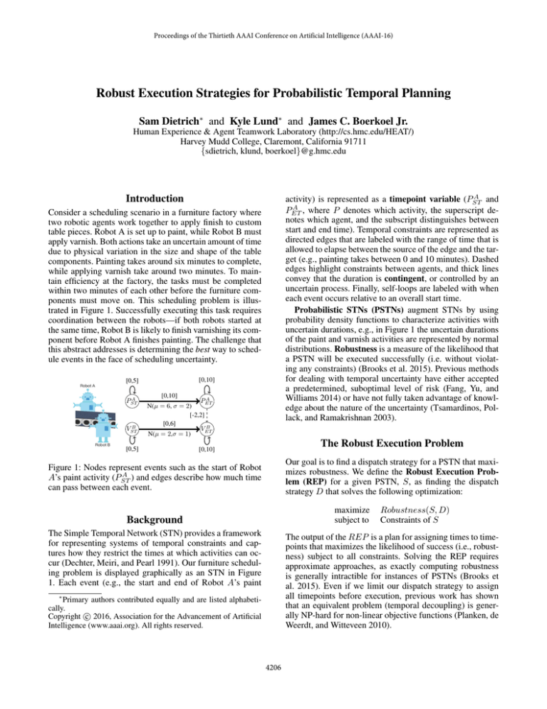
activity) is represented as a timepoint variable (PST
and
A
PET , where P denotes which activity, the superscript denotes which agent, and the subscript distinguishes between
start and end time). Temporal constraints are represented as
directed edges that are labeled with the range of time that is
allowed to elapse between the source of the edge and the target (e.g., painting takes between 0 and 10 minutes). Dashed
edges highlight constraints between agents, and thick lines
convey that the duration is contingent, or controlled by an
uncertain process. Finally, self-loops are labeled with when
each event occurs relative to an overall start time.
Probabilistic STNs (PSTNs) augment STNs by using
probability density functions to characterize activities with
uncertain durations, e.g., in Figure 1 the uncertain durations
of the paint and varnish activities are represented by normal
distributions. Robustness is a measure of the likelihood that
a PSTN will be executed successfully (i.e. without violating any constraints) (Brooks et al. 2015). Previous methods
for dealing with temporal uncertainty have either accepted
a predetermined, suboptimal level of risk (Fang, Yu, and
Williams 2014) or have not fully taken advantage of knowledge about the nature of the uncertainty (Tsamardinos, Pollack, and Ramakrishnan 2003).
Introduction
Consider a scheduling scenario in a furniture factory where
two robotic agents work together to apply finish to custom
table pieces. Robot A is set up to paint, while Robot B must
apply varnish. Both actions take an uncertain amount of time
due to physical variation in the size and shape of the table
components. Painting takes around six minutes to complete,
while applying varnish take around two minutes. To maintain efficiency at the factory, the tasks must be completed
within two minutes of each other before the furniture components must move on. This scheduling problem is illustrated in Figure 1. Successfully executing this task requires
coordination between the robots—if both robots started at
the same time, Robot B is likely to finish varnishing its component before Robot A finishes painting. The challenge that
this abstract addresses is determining the best way to schedule events in the face of scheduling uncertainty.
[0,10]
[0,5]
A
PST
B
VST
[0,10]
A
PET
N(μ = 6, σ = 2)
[-2,2]
[0,6]
B
VET
N(μ = 2,σ = 1)
[0,5]
The Robust Execution Problem
[0,10]
Our goal is to find a dispatch strategy for a PSTN that maximizes robustness. We define the Robust Execution Problem (REP) for a given PSTN, S, as finding the dispatch
strategy D that solves the following optimization:
Figure 1: Nodes represent events such as the start of Robot
A
) and edges describe how much time
A’s paint activity (PST
can pass between each event.
maximize
subject to
Background
The Simple Temporal Network (STN) provides a framework
for representing systems of temporal constraints and captures how they restrict the times at which activities can occur (Dechter, Meiri, and Pearl 1991). Our furniture scheduling problem is displayed graphically as an STN in Figure
1. Each event (e.g., the start and end of Robot A’s paint
Robustness(S, D)
Constraints of S
The output of the REP is a plan for assigning times to timepoints that maximizes the likelihood of success (i.e., robustness) subject to all constraints. Solving the REP requires
approximate approaches, as exactly computing robustness
is generally intractible for instances of PSTNs (Brooks et
al. 2015). Even if we limit our dispatch strategy to assign
all timepoints before execution, previous work has shown
that an equivalent problem (temporal decoupling) is generally NP-hard for non-linear objective functions (Planken, de
Weerdt, and Witteveen 2010).
∗
Primary authors contributed equally and are listed alphabetically.
c 2016, Association for the Advancement of Artificial
Copyright Intelligence (www.aaai.org). All rights reserved.
4206
[4.64,7.33]
[0,0]
A
PST
[4.64,7.33]
N(6,2)
A
PET
[-2,2]
B
VST
[1.35,2.67]
N(2,1)
[3.98,3.98]
B
VET
[5.33,6.64]
Figure 2: Figure 1 after applying our SREA algorithm.
Approaches for Solving the REP
Figure 3: Simulated success rates of our execution strategies
while varying interagent constraint density.
Our static robust execution algorithm (SREA) for producing an approximate solution requires finding a strategy such
that all scheduling decisions can be made before execution.
We do this by finding bounds for each contingent edge that
contain (1 − α) of the probability mass. We perform a binary search to find the minimum risk-level α that allows us
to add these bounds as constraints while retaining a valid,
executable schedule. We use an LP-formulation to both enforce all constraints and also to expand each of these bounds
some δ > 0, thus capturing even more probability mass.
The result of applying SREA to our example problem
is shown in Figure 2. The best α level found by the algorithm was 0.506, corresponding to bounds of [1.35, 2.67]
on robot A’s uncertain edge, and [4.66, 7.33] on robot B’s
uncertain edge. The LP then expanded robot B’s uncertain
edge very slightly to [4.64, 7.33]. The robustness of this
modified schedule is 24.61%, as compared to 17.21% when
the original schedule was executed with a naı̈ve “early execution” method. However, since scheduling decisions are
static, the opportunity to update decisions during execution
is lost. Our dynamic robust execution algorithm (DREA)
re-evaluates the LP whenever additional information about
uncertain events is received. The result is a dispatch algorithm that exploits favorable outcomes (e.g., a robot that
finishes early) by readjusting the remaining schedule to increase the guaranteed level of robustness. Applying DREA
increases the robustness of our example to 68.04%.
sity increased, the success rate of all approaches generally
decreased. This is expected—more dependencies between
agents means more opportunities for failure. It should be
noted that for low degrees of interagent coupling SREA performs worse than other algorithms. This is because the static
approach must restrict timepoint domains to limit risk, despite the presence of fewer constraints. At higher degrees
of coupling, SREA becomes competitive with the early execution strategy, while DREA continues to outperform other
approaches due to its ability to adjust to contingencies.
Discussion
This abstract introduces the Robust Execution Problem for
finding maximally robust execution strategies to the general
probabilistic temporal planning problem. While the REP is
likely intractable in practice, we introduce approximate solution techniques—one that can be computed statically prior
to the start of execution while providing robustness guarantees and one that dynamically adjusts to opportunities and
setbacks during execution. We show empirically that dynamically optimizing for robustness improves the likelihood
of execution success.
References
Evaluation
Brooks, J.; Reed, E.; Gruver, A.; and Boerkoel, J. C. 2015.
Robustness in probabilistic temporal planning. In Proc. of
AAAI-15, 3239–3246.
Dechter, R.; Meiri, I.; and Pearl, J. 1991. Temporal constraint networks. In Knowledge Representation, volume 49,
61–95.
Fang, C.; Yu, P.; and Williams, B. C. 2014. Chanceconstrained probabilistic simple temporal problems. In
Proc. of AAAI-14, 2264–2270.
Planken, L. R.; de Weerdt, M. M.; and Witteveen, C. 2010.
Optimal temporal decoupling in multiagent systems. In
Proc. of AAMAS-10, 789–796.
Tsamardinos, I.; Pollack, M. E.; and Ramakrishnan, S. 2003.
Assessing the Probability of Legal Execution of Plans with
Temporal Uncertainty. In ICAPS-03 Workshop on Planning
under Uncertainty.
To evaluate the efficacy of our approaches against each
other and an early execution strategy, we generated random
PSTNs with varying numbers of timepoints and constraint
characteristics. Structurally, each PSTN was composed of
several agents each with a “stick” subproblem (i.e., one with
no concurrent operations) that were subsequently connected
through interagent constraints with a check to avoid causal
loops. The pdfs associated with uncertain edges were normally distributed, with varied means and standard deviations. The problems we generated have 20 timepoints divided among 2 to 4 agents, and have 20 to 35 constraints,
of which up to 15 are uncertain. Interagent constraint density varies the proportion of constraints between agents’ sequences of actions and allows us to explore the impact of
varying degrees of interagent coupling.
As shown in Figure 3, DREA resulted in the most successful execution strategies. As interagent constraint den-
4207