Proceedings of the Twenty-Sixth AAAI Conference on Artificial Intelligence
Sensing the Air We Breathe — The OpenSense Zurich Dataset
Jason Jingshi Li1 , Boi Faltings1 , Olga Saukh2 , David Hasenfratz2 , and Jan Beutel2
1
Artificial Intelligence Laboratory, EPF Lausanne, Switzerland
Computer Engineering and Networks Laboratory, ETH Zurich, Switzerland
{jason.li, boi.faltings} @epfl.ch, {saukh, hasenfratz, beutel}@tik.ee.ethz.ch
2
Abstract
Monitoring and managing urban air pollution is a significant challenge for the sustainability of our environment. We
quickly survey the air pollution modeling problem, introduce
a new dataset of mobile air quality measurements in Zurich,
and discuss the challenges of making sense of these data.
Introduction
Urban outdoor air pollution currently accounts for up to
1.3 million deaths per year (World-Health-Organization
2011), and monitoring and managing urban air pollution is
a significant challenge for the sustainability. In this paper,
we introduce a new and growing dataset of mobile air quality measurements for the city of Zurich from the OpenSense
project. We begin with a quick survey of background knowledge on urban air pollution and existing modeling literature.
Then, we describe the data collection process and the engineering challenges of delivering high-quality measurements
using inexpensive, small, and mobile sensors. In the end, we
summarize the general problem of interpreting the collected
data and describe three reasoning approaches and detail how
they relate to each other.
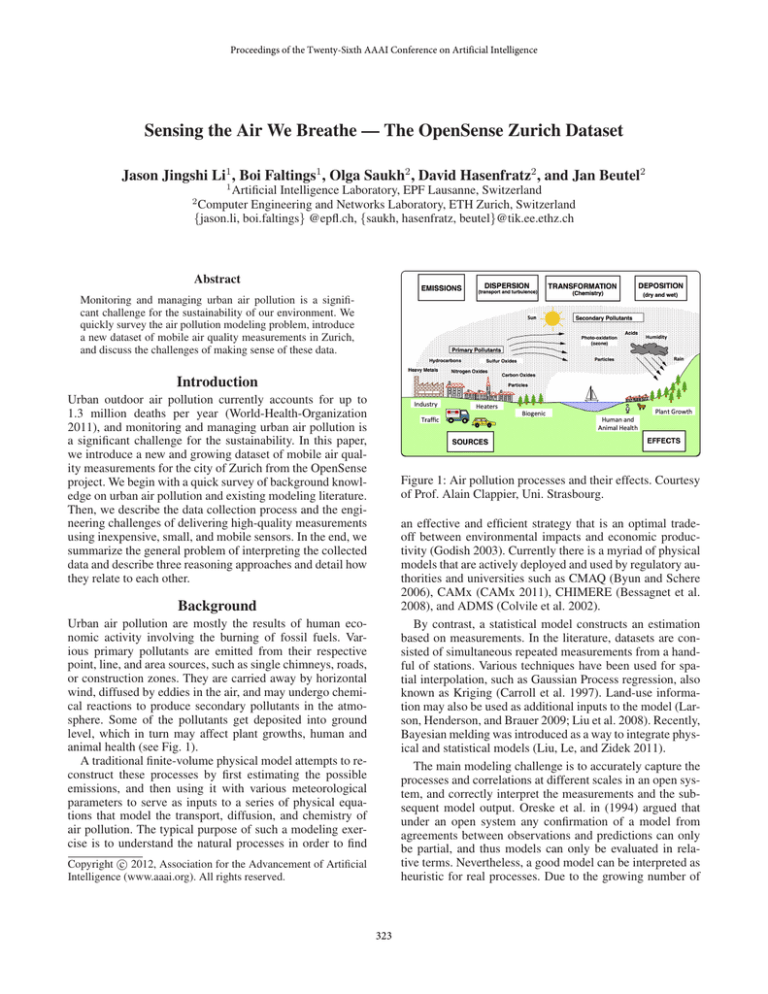
Figure 1: Air pollution processes and their effects. Courtesy
of Prof. Alain Clappier, Uni. Strasbourg.
an effective and efficient strategy that is an optimal tradeoff between environmental impacts and economic productivity (Godish 2003). Currently there is a myriad of physical
models that are actively deployed and used by regulatory authorities and universities such as CMAQ (Byun and Schere
2006), CAMx (CAMx 2011), CHIMERE (Bessagnet et al.
2008), and ADMS (Colvile et al. 2002).
By contrast, a statistical model constructs an estimation
based on measurements. In the literature, datasets are consisted of simultaneous repeated measurements from a handful of stations. Various techniques have been used for spatial interpolation, such as Gaussian Process regression, also
known as Kriging (Carroll et al. 1997). Land-use information may also be used as additional inputs to the model (Larson, Henderson, and Brauer 2009; Liu et al. 2008). Recently,
Bayesian melding was introduced as a way to integrate physical and statistical models (Liu, Le, and Zidek 2011).
The main modeling challenge is to accurately capture the
processes and correlations at different scales in an open system, and correctly interpret the measurements and the subsequent model output. Oreske et al. in (1994) argued that
under an open system any confirmation of a model from
agreements between observations and predictions can only
be partial, and thus models can only be evaluated in relative terms. Nevertheless, a good model can be interpreted as
heuristic for real processes. Due to the growing number of
Background
Urban air pollution are mostly the results of human economic activity involving the burning of fossil fuels. Various primary pollutants are emitted from their respective
point, line, and area sources, such as single chimneys, roads,
or construction zones. They are carried away by horizontal
wind, diffused by eddies in the air, and may undergo chemical reactions to produce secondary pollutants in the atmosphere. Some of the pollutants get deposited into ground
level, which in turn may affect plant growths, human and
animal health (see Fig. 1).
A traditional finite-volume physical model attempts to reconstruct these processes by first estimating the possible
emissions, and then using it with various meteorological
parameters to serve as inputs to a series of physical equations that model the transport, diffusion, and chemistry of
air pollution. The typical purpose of such a modeling exercise is to understand the natural processes in order to find
c 2012, Association for the Advancement of Artificial
Copyright Intelligence (www.aaai.org). All rights reserved.
323
(a) Tram deployment
(a) Sensor box
(b) Fixed station deployment
Figure 3: The OpenSense installations on top of a tram (a)
and next to a static reference station (b).
(b) DiSCmini
Figure 2: The OpenSense box with ozone and CO sensors (a)
and a miniature diffusion size classifier (b).
Thus, the computed calibration parameters already take sensor cross-sensitivity into account. Additionally, the sensor is
calibrated under very similar conditions as in the later deployment (e.g., same hardware and software components,
same water and dust cover) and a considerably larger number of reference measurements recorded under diverse environmental conditions can be used for calibration than what
is typically feasible in the laboratory.
Once the measurement station is deployed on the tram, we
perform automatic on-the-fly sensor calibration by exploiting the fact that public transport vehicles periodically meet
each other or pass by static reference stations. Spatially and
temporally related measurements are used to periodically
adjust calibration parameters, which is necessary to keep the
calibration up to date and filter out possible sensor aging effects. We implemented three calibration schemes described
in detail in (Hasenfratz, Saukh, and Thiele 2012). As example, by using on-the-fly calibration we are able to measure
ozone concentrations with an average error of ±2 ppb compared to the reference measurements. This is remarkable as
the accuracy of the ozone sensor is given as ±20 ppb (e2v).
Data Collection. We currently maintain two deployments
in Zurich: one on top of trams as depicted in Fig. 3(a)
and one next to a national air pollution monitoring network (NABEL) station as shown in Fig. 3(b). Both deployments are located in Zurich and are briefly described below.
The first measurement station was statically deployed
next to a reference station delivering reliable high-quality
measurements. It is used as a long-term sensor testbed running since April 2011.
Additional five stations were installed on top trams in
September 2011 and March 2012, respectively. We record
every 5 s the particulate matter pollution and every 20 s the
ozone and CO concentrations. Since the impact of mobility
on the measured concentration is still subject to investigation, we also annotate the measurements with current acceleration speeds. We plan to enhance the deployment on top
of trams to the total of 10 OpenSense stations by the end
of 2012. We also connect the gas sensors to smartphones
and gather measurements along the streets and parks with
no tram access (Hasenfratz et al. 2012).
The measurements are transmitted over GSM to our local
server running GSN (Aberer, Hauswirth, and Salehi 2006)
and are publicly available1 . Over the last six months we were
available air pollution measurements, it can be expected that
in future data-driven approaches will become more viable in
providing accurate and detailed air quality snapshots.
OpenSense Dataset
In the following, we describe our dataset based on two types
of deployments: static installation for long-term sensor testing and mobile sensor boxes on top of trams for high spatial
resolution data acquisition as shown in Fig. 3.
OpenSense System. All OpenSense stations are based on
the prototype platform developed within X-Sense (Buchli et
al. 2011) and further extended for monitoring air pollution
as depicted in Fig. 2. The core of the measurement station is
a Gumstix embedded computer running the Linux operating
system. The station supports GPRS/UMTS and WLAN for
communication and data transfers. A GPS receiver supplies
the station with precise geospatial information. Additionally,
the station is equipped with an accelerometer and has access to the tram’s door release signal to assist recognition
of halts and tram stops. The weight of the developed station
is approximately 4.5 kg and the power draw is around 40 W.
In the mobile deployment the station is continuously supplied with power from the tram. To monitor air pollution, the
OpenSense stations are equipped with ozone (e2v), CO (Alphasense), and particulate matter (Matter-Aerosol) sensors.
For all gas sensors we use water and dust covers that are
coated with a thin Teflon layer to minimize the influence of
interfering gases.
Additionally, we monitor temperature and humidity to
later convert raw sensor readings into meaningful gas concentrations and to compute the sensor calibration parameters. All sensor readings are position and time stamped.
Data Calibration. There are two common approaches for
the calibration of gas sensors that are intended for urban air
pollution monitoring. The calibration can take place either
in the laboratory using reference gas mixtures (Choi et al.
2009) or in the field by placing a sensor close to a static highquality reference station delivering reliable pollution concentrations (Kamionka, Breuil, and Pijolat 2006). We use
the second approach for sensor calibration, since this way
we can observe the sensor performance under a wide range
of weather conditions and in the presence of other gases.
1
324
http://data.opensense.ethz.ch
References
(a) Ozone
Aberer, K.; Hauswirth, M.; and Salehi, A. 2006. A middleware for
fast and flexible sensor network deployment. In VLDB.
Alphasense. 2011. COAF sensor on a digital transmitter board.
Bessagnet, B.; Menut, L.; Curci, G.; Hodzic, A.; Guillaume, B.;
Liousse, C.; Moukhtar, S.; Pun, B.; Seigneur, C.; and Schulz, M.
2008. Regional modeling of carbonaceous aerosols over europe—
focus on secondary organic aerosols. In Springer Journal of Atmospheric Chemistry.
Buchli, B.; Yuecel, M.; Lim, R.; Gsell, T.; and Beutel, J. 2011.
Demo abstract: Feature-rich platform for WSN design space exploration. In ACM/IEEE IPSN.
Byun, D., and Schere, K. L. 2006. Review of the governing
equations, computational algorithms, and other components of the
models-3 community multiscale air quality (CMAQ) modeling system. In ASME Applied Mechanics Reviews.
CAMx. 2011. Comprehensive air quality model with extensions.
In http:// www.camx.com.
Carroll, R.; Chen, R.; George, E.; Li, T.; Newton, H.; Schmiediche,
H.; and Wang, N. 1997. Ozone exposure and population density in
harris county, texas. In JSTOR JASA.
Choi, S.; Kim, N.; Cha, H.; and Ha, R. 2009. Micro sensor node for
air pollutant monitoring: Hardware and software issues. In MEMS
Sensors.
Colvile, R. N.; Woodfield, N. K.; Carruthers, D. J.; Fisher, B. E. A.;
Rickard, A.; Neville, S.; and Hughes, A. 2002. Uncertainty in
dispersion modelling and urban air quality mapping. In Elsevier
Environmental Science and Policy.
e2v. 2011. MiCS-OZ-47 ozone sensing head with smart transmitter
board.
Godish, T. 2003. Air quality. In CRC Press.
Hasenfratz, D.; Saukh, O.; Sturzenegger, S.; and Thiele, L. 2012.
Participatory air pollution monitoring using smartphones. In Mobile Sensing.
Hasenfratz, D.; Saukh, O.; and Thiele, L. 2012. On-the-fly calibration of low-cost gas sensors. In Springer EWSN.
Kamionka, M.; Breuil, P.; and Pijolat, C. 2006. Calibration of a
multivariate gas sensing device for atmospheric pollution measurement. In Elsevier Sensors and Actuators B: Chemical.
Keller, M., and Beutel, J. 2011. Demo abstract: Efficient data
retrieval for interactive browsing of large sensor network data sets.
In ACM/IEEE IPSN.
Larson, T.; Henderson, S. B.; and Brauer, M. 2009. Mobile monitoring of particle light absorption coefficient in an urban area as
a basis for land use regression. In ACS Publications Enviromental
Science and Technology.
Liu, Y.; Guo, H.; Mao, G.; and Yang, P. 2008. A bayesian hierarchical model for urban air quality prediction under uncertainty. In
Elsevier Atmospheric Environment.
Liu, Z.; Le, N. D.; and Zidek, J. V. 2011. An empirical assessment
of bayesian melding for mapping ozone pollution. In John Wiley &
Sons, Ltd. Environmetrics.
Matter-Aerosol. 2011. DiSCmini: Miniature diffusion size classifier.
Oreskes, N.; Shrader-Frechette, K.; and Belitz, K. 1994. Verification, validation, and confirmation of numerical models in the earth
sciences. In Science.
World-Health-Organization. 2011. Air quality and health. In Fact
Sheet No. 313.
(b) PM
Figure 4: Web-based interactive data browsing through the
datasets of ozone and PM measurements in Zurich.
able to gather over 3 million data points with our two deployments. To conveniently access the data, we use locationbased data aggregation and time-based data caching for
fast and efficient data access and interactive data browsing (Keller and Beutel 2011) as illustrated in Fig. 4 for ozone
and particulate matter measurements.
The Challenge
For a given deployment of air quality sensors, there are a
few things we would typically like to infer from the resulting dataset, such as what are the pollution levels at some
space and time, where the pollution came from, and how we
could better place the sensors to get a clearer picture. Here
we summarize the general challenge of making sense from
the data concerning three classes of reasoning tasks and discuss some of the current approaches for solving these tasks.
Forward Reasoning. The first type of reasoning tasks is to
create spatial and temporal interpolations, which involves
deducing more information from the data based on certain
assumptions and inference rules. Typical queries include
pollution levels for locations where no sensors are available, likely pollution levels at a certain point in the future,
or whether to place advanced warnings of dangerous pollution levels. This is the predominant task for most of the
current air pollution models.
Backward Reasoning. The second type of reasoning tasks
involves working backwards for likely explanations to the
observed measurements. They may include identifying unknown or unexpected emission sources, or identify the dispersion mechanisms. It would require developing a causal
model for air pollution. Unlike forward reasoning, this appears to be a more complex task due to uncertainties.
Meta-Reasoning. The third type of reasoning tasks concerns with how to manage the sensing resources in order to
better accomplish the forward or backward reasoning tasks.
This may involve sensor placement, sensor scheduling, or a
mixture of both. In the case of community sensing, another
challenge is how to engineer the incentives such, that agents
are driven to optimize the sensing quality.
Acknowledgements. The authors thank Christoph Walser
for the technical support. This work was part of the
Opensense project funded by the Nanotera.ch program.
325