Proceedings of the Fifth Annual Symposium on Combinatorial Search
E-Graphs: Bootstrapping Planning with Experience Graphs∗
Mike Phillips
Benjamin Cohen
Sachin Chitta
Maxim Likhachev
mlphilli@andrew.cmu.edu
Carnegie Mellon University
bcohen@seas.upenn.edu
University of Pennsylvania
sachinc@willowgarage.com
Willow Garage
maxim@cs.cmu.edu
Carnegie Mellon University
Abstract
In this paper, we develop an online motion planning approach which learns from its planning episodes (experiences) a graph, an Experience Graph. On the theoretical side, we show that planning with Experience graphs
is complete and provides bounds on suboptimality with
respect to the graph that represents the original planning problem. Experimentally, we show in simulations
and on a physical robot that our approach is particularly
suitable for higher-dimensional motion planning tasks
such as planning for two armed mobile manipulation.
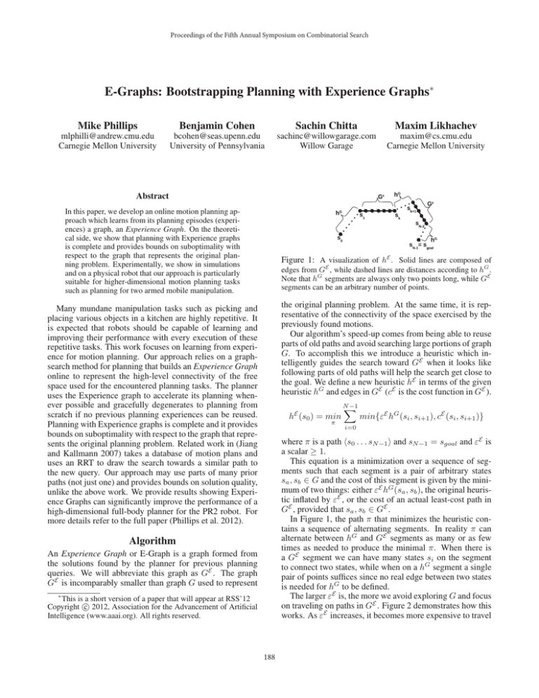
Figure 1: A visualization of hE . Solid lines are composed of
edges from GE , while dashed lines are distances according to hG .
Note that hG segments are always only two points long, while GE
segments can be an arbitrary number of points.
the original planning problem. At the same time, it is representative of the connectivity of the space exercised by the
previously found motions.
Our algorithm’s speed-up comes from being able to reuse
parts of old paths and avoid searching large portions of graph
G. To accomplish this we introduce a heuristic which intelligently guides the search toward GE when it looks like
following parts of old paths will help the search get close to
the goal. We define a new heuristic hE in terms of the given
heuristic hG and edges in GE (cE is the cost function in GE ).
Many mundane manipulation tasks such as picking and
placing various objects in a kitchen are highly repetitive. It
is expected that robots should be capable of learning and
improving their performance with every execution of these
repetitive tasks. This work focuses on learning from experience for motion planning. Our approach relies on a graphsearch method for planning that builds an Experience Graph
online to represent the high-level connectivity of the free
space used for the encountered planning tasks. The planner
uses the Experience graph to accelerate its planning whenever possible and gracefully degenerates to planning from
scratch if no previous planning experiences can be reused.
Planning with Experience graphs is complete and it provides
bounds on suboptimality with respect to the graph that represents the original planning problem. Related work in (Jiang
and Kallmann 2007) takes a database of motion plans and
uses an RRT to draw the search towards a similar path to
the new query. Our approach may use parts of many prior
paths (not just one) and provides bounds on solution quality,
unlike the above work. We provide results showing Experience Graphs can significantly improve the performance of a
high-dimensional full-body planner for the PR2 robot. For
more details refer to the full paper (Phillips et al. 2012).
E
h (s0 ) = min
π
N
−1
X
min{εE hG (si , si+1 ), cE (si , si+1 )}
i=0
where π is a path hs0 . . . sN −1 i and sN −1 = sgoal and εE is
a scalar ≥ 1.
This equation is a minimization over a sequence of segments such that each segment is a pair of arbitrary states
sa , sb ∈ G and the cost of this segment is given by the minimum of two things: either εE hG (sa , sb ), the original heuristic inflated by εE , or the cost of an actual least-cost path in
GE , provided that sa , sb ∈ GE .
In Figure 1, the path π that minimizes the heuristic contains a sequence of alternating segments. In reality π can
alternate between hG and GE segments as many or as few
times as needed to produce the minimal π. When there is
a GE segment we can have many states si on the segment
to connect two states, while when on a hG segment a single
pair of points suffices since no real edge between two states
is needed for hG to be defined.
The larger εE is, the more we avoid exploring G and focus
on traveling on paths in GE . Figure 2 demonstrates how this
works. As εE increases, it becomes more expensive to travel
Algorithm
An Experience Graph or E-Graph is a graph formed from
the solutions found by the planner for previous planning
queries. We will abbreviate this graph as GE . The graph
GE is incomparably smaller than graph G used to represent
∗
This is a short version of a paper that will appear at RSS’12
c 2012, Association for the Advancement of Artificial
Copyright Intelligence (www.aaai.org). All rights reserved.
188
(a) εE = 1
(b) εE = 2
(c) εE → ∞
Figure 2: Shortest π according to hE as εE changes. The dark
solid lines are paths in GE while the dark dashed lines are the
heuristic’s path π. Note as εE increases, the heuristic prefers to
travel on GE . The light gray circles and lines show the graph G
and the filled in gray circles represent the expanded states under
the guidance of the heuristic.
(a) Bootstrap goals
(b) One of the test sets
Figure 3: Full-body planning in a warehouse
Table 1: Weighted A* to E-Graph Ratios on Warehouse Environ-
off of GE causing the heuristic to guide the search along
parts of GE . In Figure 2a, the heuristic ignores the graph GE
because without inflating hG at all, following edges in GE
will never be the cheaper option. On the other hand as εE
increases, the heuristic uses more and more of GE (Figure
2b, 2c). This figure also shows how during the search, by
following old paths, we can avoid obstacles and have far
fewer expansions. The expanded states are shown as filled
in gray circles, which change based on how the hE is biased
by εE .
We run weighted A* without re-expansions (Likhachev,
Gordon, and Thrun 2003). In addition to using the edges in
G, we add two additional types of successors: shortcuts and
snap motions. Also, instead of using the heuristic hG , we
use our new heuristic hE , inflated by εw ≥ 1. Shortcut successors are generated when expanding a state s ∈ GE . They
use GE to jump to a state that is closest to sgoal according
to the heuristic. The shortcuts allow the planner to quickly
get near the goal without having to re-generate paths in GE .
Finally, for environments that can support it, we introduce
snap motions, which are dynamically generated successors
for states that are very close to GE . These motions attempt
to connect these close states directly to a nearby state on GE
so a shortcut on it may be used.
Since no edges are removed from the graph (we only add)
and we are searching the graph with Weighted A* (a complete planner), if a solution exists on the original graph, our
algorithm will find it. Furthermore, our planner provides a
bound on the suboptimality of the solution cost with respect
to the original graph.
ment (100 goals per set)
Set
1
2
3
4
5
mean time(s)
18.40
17.74
224.83
24.30
16.69
std dev time(s)
39.94
51.24
1674.12
155.42
72.41
mean expands
206
231
1562
142
193
mean cost
0.63
0.60
0.63
0.64
0.62
region, we first bootstrap it with 45 uniformly distributed
goals (split between the pallet and shelves). The bootstrap
goals and the resultant GE after processing them are shown
in Figure 3a. We use a 3D Dijkstra search to implement the
hE for a sphere inscribed in the carried object starting from
its goal position. In all experiments, εw = 2 and εE = 10
resulting in a suboptimality bound of 20. The results were
compared against regular Weighted A* with εw = 20 so
both approaches have the same bound.
Table 2: 10% Most difficult Cases on Warehouse Environment (10
goals per set)
Set
Mean Time Ratio
1
122.68
2
128.12
3
2157.14
4
200.80
5
112.17
A set of 100 random goals (with varying positions and
yaws of the object) alternating between the pallet and
shelves were then specified to the planner. This process was
repeated 5 times with GE cleared before running each set of
100 goals. Table 1 compares the two approaches by examining the ratio between planning times for Weighted A* and
the E-Graph approach. The data indicates that planning with
E-Graphs is almost 20 times faster. On average, 94% of the
edges on a path produced by our planner were recycled from
GE . Table 2 compares the 10% hardest goals (the ones that
took the Weighted A* the longest to solve) showing that our
approach is over 100 times faster on such difficult goals.
Theorem 1. For a finite graph G, the planner terminates,
and the solution it returns is guaranteed to be no worse than
εw · εE times the optimal solution cost in graph G.
References
Experimental Results
Jiang, X., and Kallmann, M. 2007. Learning humanoid
reaching tasks in dynamic environments. In IEEE International Conference on Intelligent Robots and Systems.
Likhachev, M.; Gordon, G.; and Thrun, S. 2003. ARA*:
Anytime A* with provable bounds on sub-optimality. In Advances in Neural Information Processing Systems (NIPS).
Phillips, M.; Cohen, B.; Chitta, S.; and Likhachev, M. 2012.
E-graphs: Bootstrapping planning with experience graphs.
In Proceedings of the Robotics: Science and Systems (RSS).
One of our experiments is modeled on an industrial warehouse where the robot must move upright objects from a
pallet to a shelving unit. The 10 dimensional planning problem includes moving the base and the two arms which are
rigidly attached to the object. Since our planner improves
in performance with repeated attempts in a particular spatial
We thank Willow Garage for their support of this work. This
research was also sponsored by ARL, under the Robotics CTA program grant W911NF-10-2-0016.
189