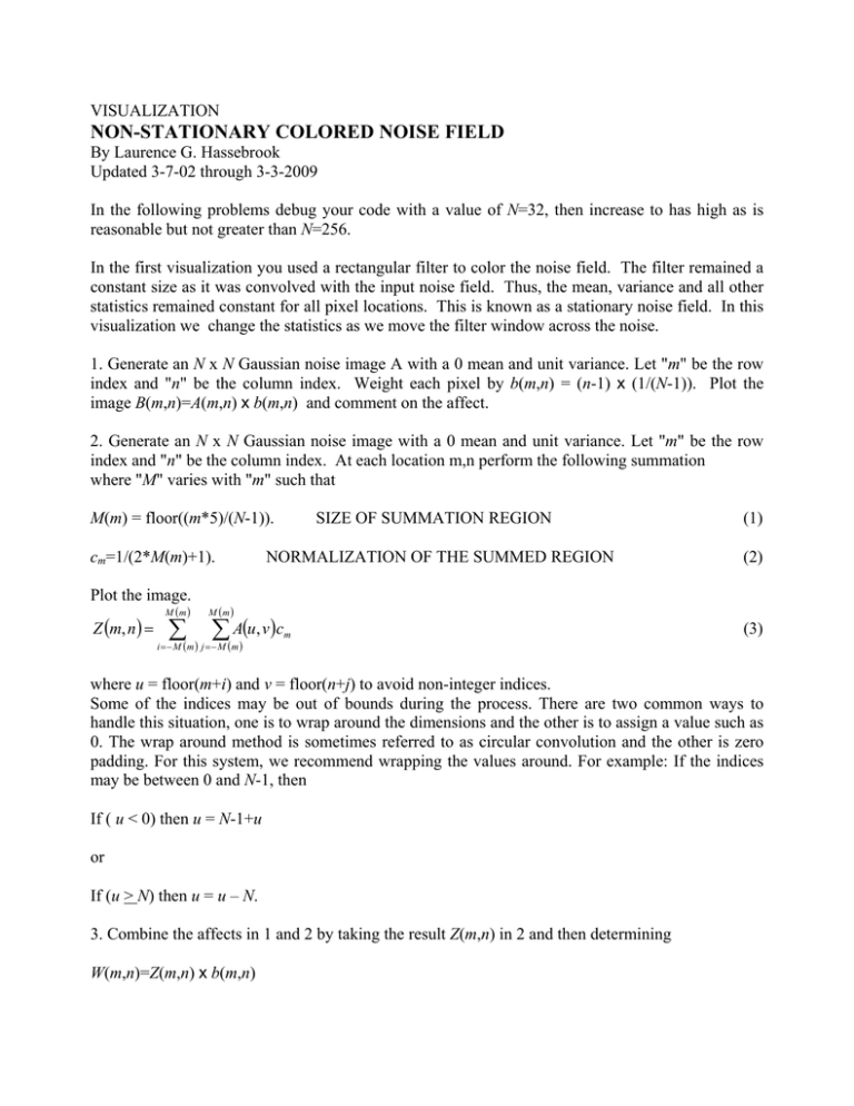
VISUALIZATION
NON-STATIONARY COLORED NOISE FIELD
By Laurence G. Hassebrook
Updated 3-7-02 through 3-3-2009
In the following problems debug your code with a value of N=32, then increase to has high as is
reasonable but not greater than N=256.
In the first visualization you used a rectangular filter to color the noise field. The filter remained a
constant size as it was convolved with the input noise field. Thus, the mean, variance and all other
statistics remained constant for all pixel locations. This is known as a stationary noise field. In this
visualization we change the statistics as we move the filter window across the noise.
1. Generate an N x N Gaussian noise image A with a 0 mean and unit variance. Let "m" be the row
index and "n" be the column index. Weight each pixel by b(m,n) = (n-1) x (1/(N-1)). Plot the
image B(m,n)=A(m,n) x b(m,n) and comment on the affect.
2. Generate an N x N Gaussian noise image with a 0 mean and unit variance. Let "m" be the row
index and "n" be the column index. At each location m,n perform the following summation
where "M" varies with "m" such that
M(m) = floor((m*5)/(N-1)).
cm=1/(2*M(m)+1).
Plot the image.
Z (m, n ) =
M (m )
∑
SIZE OF SUMMATION REGION
NORMALIZATION OF THE SUMMED REGION
(1)
(2)
M (m )
∑ A(u, v )c
i = − M (m ) j = − M (m )
m
(3)
where u = floor(m+i) and v = floor(n+j) to avoid non-integer indices.
Some of the indices may be out of bounds during the process. There are two common ways to
handle this situation, one is to wrap around the dimensions and the other is to assign a value such as
0. The wrap around method is sometimes referred to as circular convolution and the other is zero
padding. For this system, we recommend wrapping the values around. For example: If the indices
may be between 0 and N-1, then
If ( u < 0) then u = N-1+u
or
If (u > N) then u = u – N.
3. Combine the affects in 1 and 2 by taking the result Z(m,n) in 2 and then determining
W(m,n)=Z(m,n) x b(m,n)
Plot W and comment.
4. Use functions like surf, surface, shading and/or light to treat the image in 3 as a 3-D surface
topology. Plot results which should show the affects of gradually changing noise “color” and
intensity.