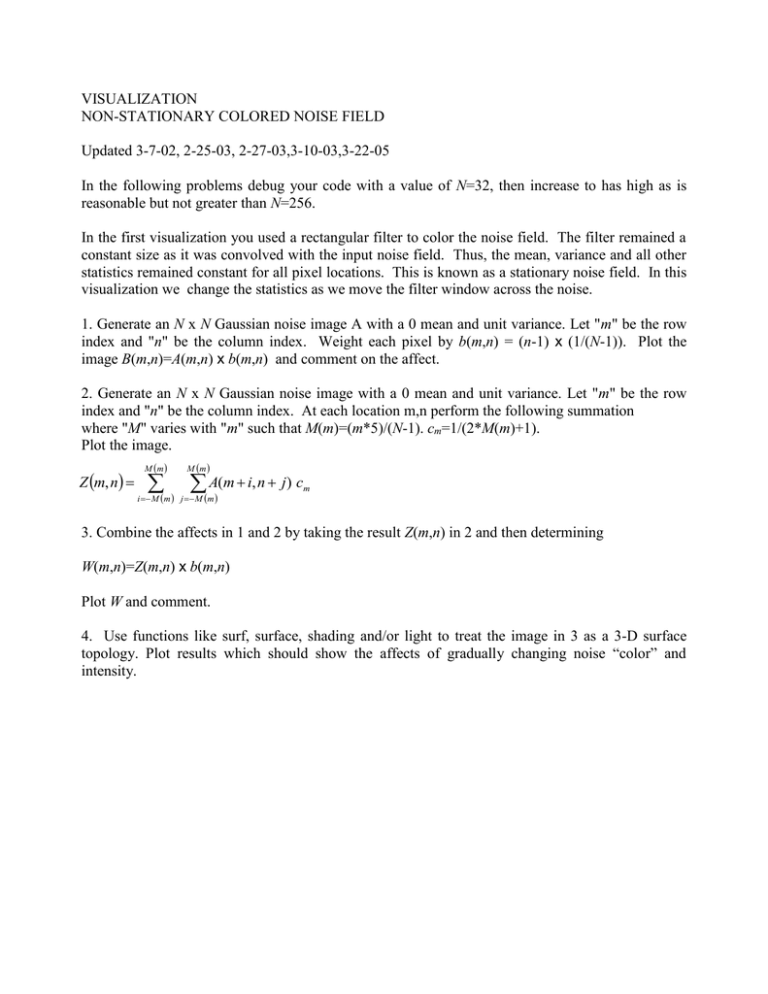
VISUALIZATION
NON-STATIONARY COLORED NOISE FIELD
Updated 3-7-02, 2-25-03, 2-27-03,3-10-03,3-22-05
In the following problems debug your code with a value of N=32, then increase to has high as is
reasonable but not greater than N=256.
In the first visualization you used a rectangular filter to color the noise field. The filter remained a
constant size as it was convolved with the input noise field. Thus, the mean, variance and all other
statistics remained constant for all pixel locations. This is known as a stationary noise field. In this
visualization we change the statistics as we move the filter window across the noise.
1. Generate an N x N Gaussian noise image A with a 0 mean and unit variance. Let "m" be the row
index and "n" be the column index. Weight each pixel by b(m,n) = (n-1) x (1/(N-1)). Plot the
image B(m,n)=A(m,n) x b(m,n) and comment on the affect.
2. Generate an N x N Gaussian noise image with a 0 mean and unit variance. Let "m" be the row
index and "n" be the column index. At each location m,n perform the following summation
where "M" varies with "m" such that M(m)=(m*5)/(N-1). cm=1/(2*M(m)+1).
Plot the image.
Z m, n 
M m 

M m 
 A(m  i, n  j) c
i  M m  j  M m 
m
3. Combine the affects in 1 and 2 by taking the result Z(m,n) in 2 and then determining
W(m,n)=Z(m,n) x b(m,n)
Plot W and comment.
4. Use functions like surf, surface, shading and/or light to treat the image in 3 as a 3-D surface
topology. Plot results which should show the affects of gradually changing noise “color” and
intensity.