Speeding up Inference in Markovian Models
Theodore Charitos, Peter de Waal and Linda C. van der Gaag
Institute of Information and Computing Sciences, Utrecht University
P.O Box 80.089, 3508 TB Utrecht, The Netherlands
{theodore,waal,linda}@cs.uu.nl
Abstract
Sequential statistical models such as dynamic Bayesian networks and hidden Markov models more specifically, model
stochastic processes over time. In this paper, we study for
these models the effect of consecutive similar observations
on the posterior probability distribution of the represented
process. We show that, given such observations, the posterior distribution converges to a limit distribution. Building
upon the rate of the convergence, we further show that, given
some wished-for level of accuracy, part of the inference can
be forestalled, thereby reducing the computational requirements upon runtime.
Introduction
Sequential statistical models for reasoning about stochastic
processes include hidden Markov models (HMMs) and dynamic Bayesian networks (DBNs); when these models satisfy the Markovian property, where the future state of the
process is assumed to be independent of the past state given
its present state, we call them Markovian. Markovian models represent the dynamics of a discrete-time process by explicitly specifying a stochastic transition rule for the change
of the state of the process from time n to time n + 1. DBNs
(Dean and Kanazawa, 1989; Murphy 2002) model the interactions among several dynamic variables and in essence
constitute an extension of HMMs which capture the dynamics of a single variable (Rabiner 1989). Applications of
Markovian models include medical diagnosis, speech recognition, computational biology and computer vision.
Exact inference in Markovian models is computationally
hard, especially since all variables tend to become correlated over time. The computational requirements of algorithms for exact inference in fact are high enough to render them infeasible in practice. In this paper, we will show
that the nature of the observations obtained may help reduce
the requirements of these algorithms. We will show more
specifically that, after a certain number of consecutive similar observations, the posterior distribution of the stochastic
process has converged to a limit distribution within some
level of accuracy. Continuing to obtain similar observations
will not alter the distribution beyond this level, and no further inference is required. The total number of time steps
c 2005, American Association for Artificial IntelliCopyright °
gence (www.aaai.org). All rights reserved.
£
G = 0.13
P =
·
0.95
0.15
0.87
¤
¸
·
0.708
0.05
OSA =
0.55
0.85
¸
·
0.292
0.56
OBT =
0.45
0.028
0.24
0.95
¸
0.2
0.022
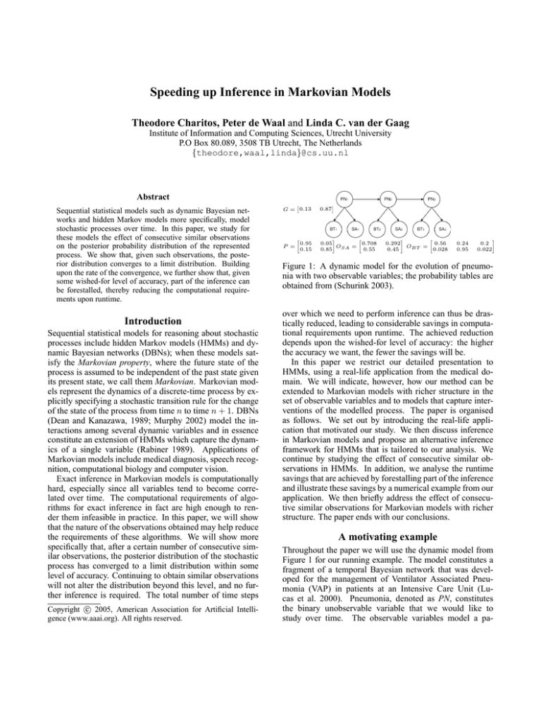
Figure 1: A dynamic model for the evolution of pneumonia with two observable variables; the probability tables are
obtained from (Schurink 2003).
over which we need to perform inference can thus be drastically reduced, leading to considerable savings in computational requirements upon runtime. The achieved reduction
depends upon the wished-for level of accuracy: the higher
the accuracy we want, the fewer the savings will be.
In this paper we restrict our detailed presentation to
HMMs, using a real-life application from the medical domain. We will indicate, however, how our method can be
extended to Markovian models with richer structure in the
set of observable variables and to models that capture interventions of the modelled process. The paper is organised
as follows. We set out by introducing the real-life application that motivated our study. We then discuss inference
in Markovian models and propose an alternative inference
framework for HMMs that is tailored to our analysis. We
continue by studying the effect of consecutive similar observations in HMMs. In addition, we analyse the runtime
savings that are achieved by forestalling part of the inference
and illustrate these savings by a numerical example from our
application. We then briefly address the effect of consecutive similar observations for Markovian models with richer
structure. The paper ends with our conclusions.
A motivating example
Throughout the paper we will use the dynamic model from
Figure 1 for our running example. The model constitutes a
fragment of a temporal Bayesian network that was developed for the management of Ventilator Associated Pneumonia (VAP) in patients at an Intensive Care Unit (Lucas et al. 2000). Pneumonia, denoted as PN, constitutes
the binary unobservable variable that we would like to
study over time. The observable variables model a pa-
BT
<36.0
normal
SA
6
6
¦
r
r
r
¦
¦
¦
¦
¦
¦
r
r
r
r
2
4
¦
¦
¦
¦
r
r
r
r
r
14
16
18
20
22
yes
no
>38.5
24
¦
6
8
10
12
-
time (hrs)
Figure 2: The dataset for patient Id.1015, May 18, where •
is used for a BT observation and ¦ for an SA observation.
24:00-12:00
14:00-22:00
BT=normal
BT=> 38.5
BT=normal, SA=no
BT=normal, SA=yes
BT=> 38.5, SA=yes
SA=no
SA=yes
2:00-4:00
6:00-22:00
2:00-4:00
6:00-12:00
14:00-22:00
Table 1: The sequences of consecutive similar observations per variable and for both variables combined, from the
dataset for patient Id.1015, May 18.
tient’s body temperature, denoted as BT, with the values
{> 38.5 ◦ C, normal, < 36.0 ◦ C}, and sputum amount, denoted as SA, with the values {yes, no}. The observable variables are measured every two hours. As an example, Figure
2 illustrates the data obtained for a specific patient on a specific day.
From Figure 2 we note that, within the data, two sequences of consecutive similar observations can be discerned per variable; for both variables combined, three such
sequences are found. Table 1 summarises these findings. We
now are interested in determining whether we need to use all
the available data to establish the probability distribution of
the variable PN within reasonable accuracy. For example,
using the tables from Figure 1, we compute the probability
of pneumonia at time 22:00 to be p(P N = yes) = 0.9951.
This probability does not differ much from the probability
at time 20:00 which is p(P N = yes) = 0.9950, nor from
that at time 18:00 which is p(P N = yes) = 0.9935. Since
after a specific number of similar consecutive observations
the probability distribution of the dynamic process does not
change much, it is worthwhile to investigate whether we can
forestall part of the inference.
Markovian models
We review some basic concepts from the theory of Markovian models, and present an inference framework for HMMs
that is tailored to our analysis.
Basic notions
A hidden Markov model can be looked upon as an extension
of a finite Markov chain, by including observable variables
that depend on the hidden variable. We use Xn to denote the
hidden variable, with states SX = {1, 2, . . . , m}, m ≥ 1,
at time n. We denote the prior probability distribution of
the hidden variable at time 1 by G, with probabilities gi =
p(X1 = i). The transition behaviour of a Markov chain
is generally represented by a matrix P of transition probabilities. We consider only homogeneous Markov chains in
which the transition probabilities do not depend on time, and
define pij = p(Xn+1 = j | Xn = i) for every n ≥ 1. We
assume that the diagonal of the transition matrix has nonzero elements only, that is, we assume that it is possible for
each state to persist. We denote the observable variables by
Yn , with values SY = {1, 2, . . . , r}, r ≥ 1. The observations are generated from the state of the hidden variable
according to a time-invariant probability distribution matrix
O, where the (i, j)-th entry gives, for each n ≥ 1, the probability of observing Yn = j given that the hidden variable
Xn is in state i, that is, oij = p(Yn = j | Xn = i).
A dynamic Bayesian network can be looked upon as an
extension of an HMM, that captures a process that involves
a collection of hidden and observable variables. The set of
variables Vn of the DBN is split into three mutually exclusive and collectively exhaustive sets In , Xn , Yn , where the
sets In and Yn constitute the input and output variables at
time n, and Xn includes the hidden variables. The joint
probability distribution over the variables per time step is
captured in a factorised way by a graphical model.
Inference in Markovian models
When applying Markovian models, usually the probability
distributions of the hidden variables are computed using an
inference algorithm. Three different types of inference are
distinguished, namely monitoring, smoothing and forecasting. Monitoring is the task of computing the probability distributions for Xn at time n given observations up to and including time n. Smoothing (or diagnosis) is the task of computing the probability distributions for Xn at time n given
observations from the future up to time N , where N > n.
Finally, forecasting is the task of predicting the probability
distributions of Xn at time n given observations about the
past up to and including time N , where N < n. Rabiner
(Rabiner 1989) introduced an efficient recursive scheme,
called the Forward-Backward algorithm, for performing exact inference in HMMs, while Murphy (Murphy 2002) presented and reviewed several algorithms for exact and approximate inference in DBNs.
We propose an alternative framework for inference in
HMMs that is suited to our analysis of the effect of consecutive similar observations. We denote by DN the dataset
of observations up to and including time N ; we assume that
there are no missing values in DN . We further denote by
OM (j) = diag(O1j , . . . , Omj ), j = 1, . . . , r, the diagonal
matrix constructed from the jth column of the observation
matrix O; we call this matrix the observation column matrix
for j. The present row vector for time n now is defined as
P Vn (i) = p(Xn = i | Dn ), i = 1, . . . , m, and is computed
recursively as follows:
• at time 1, if there is an observation j, we take
P V1 = G · OM (j);
same value j is observed from time n up to and including
time N for some n < N ; the number of consecutive similar
observations thus is kj = N − (n − 1). Using our inference
framework, the present row vector P VN is computed to be
P VN = αkj · P Vn−1 · (P · OM (j))kj
Forward influence
Backward influence
Figure 3: Arc reversal in a HMM.
• at time n = 2, . . . , N , if there is an observation j, we take
P Vn = P Vn−1 · P · OM (j).
In each step, we normalise the vector P Vn by dividing by
P
m
i=1 P Vn (i).
For forecasting the probability distribution of the hidden
variable Xn for some time n > N , we define the future row
vector F Vn,N (i) = p(Xn = i | DN ), i = 1, . . . , m. The
future row vector is computed as F Vn,N = P VN · P n−N .
For computing a smoothed probability distribution for
some time n < N , we define the backward row vector
BVn,N (i) = p(Xn = i | DN ), i = 1, . . . , m. The backward row vector is computed by performing evidence absorption and arc reversal (Shachter 1988) in the model; Figure 3 illustrates the basic idea. The states of the variable Xn
affect the probability distribution of the variable Xn+1 via
the transition matrix P . By using Bayes’ theorem
p(Xn+1 | Xn ) · p(Xn )
(1)
p(Xn | Xn+1 ) =
p(Xn+1 )
and arc reversal, we find that the states of the variable Xn+1
affect the probability distribution of the variable Xn via the
matrix AP n+1,n , where APijn+1,n = p(Xn = j | Xn+1 =
i). The matrix AP n+1,n is established for n = 1, . . . , N − 1
from
• p(Xn ) = P Vn ;
• p(Xn+1 ) = p(Xn ) · P ;
• AP n+1,n is computed using equation (1).
The backward row vector BVn,N then is computed recursively from
• BVN,N = P VN ;
• for n = N − 1, . . . , 1, BVn,N = BVn+1,N · AP n+1,n .
Again, weP
normalise the vector BVn,N in each step by dim
viding by i=1 BVn,N (i).
Similar observations
We analyse the effect of observing consecutive similar values for an observable variable on the probability distribution
of the hidden variable. More specifically, we are interested
in the convergence behaviour of the posterior distribution of
Xn in terms of the number kj of consecutive observations j.
We will argue that, given a specific kj , observing more similar values will not alter the probability distribution of the
hidden variable beyond a given level of accuracy.
We consider a hidden Markov model with a single observable variable and an associated dataset DN . Suppose that the
= αkj · P Vn−1 · (Rj )kj
(2)
where αkj is a normalization constant that depends on kj
and Rj is the square matrix Rj = P · OM (j). We use equation (2) to study the convergence of the present row vector to
a limit distribution. More specifically, we would like to estimate the number kj of consecutive observations such that
|P Vkj +1 − P Vkj |∞ ≤ θ
where θ > 0 is a predefined level of accuracy and
|w|∞ ≡ maxi |wi | denotes the L∞ norm of a vector w =
(w1 , . . . , wm ). We then have that observing more than kj
consecutive similar values will add no extra information to
the probability distribution of the hidden variable and no further inference needs to be performed.
To establish the convergence behaviour of the present row
vector and of the matrix Rj more specifically, we will build
upon the notion of spectral radius, where the spectral radius
ρ(A) of a square matrix A is defined as ρ(A) ≡ max{|λ| :
λ is an eigenvalue of A}. The following theorem (Horn
and Johnson, 1990, Theorem 5.6.12) now reviews a necessary and sufficient condition for the convergence of reflexive
multiplication of a square matrix in terms of its spectral radius.
Theorem 1 Let A be a square matrix. Then, limk→∞ Ak =
0 if and only if ρ(A) < 1.
To study the spectral radius of the matrix Rj , we recall that
it is the product of a stochastic matrix P and the nonnegative
diagonal observation column matrix OM (j). The following
proposition now shows that ρ(Rj ) ≤ 1.
Proposition 1 Let A be a stochastic matrix and let B be a
diagonal matrix. Then, ρ(A · B) ≤ ρ(B).
Proof: From (Horn and Johnson, 1990, Theorem 5.6.9) we
have that for any square matrix A, it holds that ρ(A) ≤ kAk,
where k¦k is any matrix norm. From this property we have
that ρ(A · B) ≤ kA · Bk. Now, any matrix norm satisfies
the submultiplicative axiom which states that kA · Bk ≤
kAk · kBk. Hence, ρ(A · B) ≤ kAk · kBk. If we choose the
maximum row sum matrix norm k¦k∞ defined on A as
n
X
kAk∞ ≡ max
|aij |,
i
j=1
we have that kAk∞ = ρ(A) = 1 and kBk∞ = ρ(B). The
property stated in the proposition now follows directly. ¤
From Proposition 1 we conclude for the spectral radius of the matrix Rj that ρ(Rj ) ≤ ρ(OM (j)). We
further find that ρ(Rj ) = 1 only if OM (j) is the identity
matrix, which basically means that the observation j is
deterministically related with the hidden state. For any
non-trivial observation column matrix, therefore, we have
that ρ(Rj ) < 1. From Theorem 1 we can now conclude
k
that limkj →∞ Rj j = 0. Note that from this property we
have that the present row vector P VN converges to some
limit distribution. The property, however, does not give
any insight in this limit distribution nor in the rate of the
convergence. For this purpose we can build upon the
following theorem, known as Perron’s theorem (Horn and
Johnson, 1990, Theorem 8.2.11), which provides a limit
matrix for [ρ(Rj )−1 · Rj ]kj .
Theorem 2 (Perron’s theorem) Let A be a square matrix
with positive elements. Then, limk→∞ [ρ(A)−1 · A]k = LA
where LA ≡ x · y T , with A · x = ρ(A) · x, AT · y =
ρ(A) · y, x > 0, y > 0, and xT · y = 1.
By rewriting equation (2) into
P VN = αkj · P Vn−1 · ρ(Rj )kj (Rj /ρ(Rj ))kj
we now apply Perron’s theorem to establish the limit distribution for the vector P VN .
Theorem 3 Let ckj ≡ αkj ·ρ(Rj )kj , where αkj , kj and Rj
are as in equation (2). Then, limkj →∞ ckj = c for some
constant c > 0, and limkj →∞ P VN = c · P Vn−1 · LRj ,
where LRj is as defined in Theorem 2.
Proof: By definition we have that
ckj = αk · ρ(Rj )kj = P
ρ(Rj )kj
i (P Vn−1
k
· Rj j )(i)
From Theorem 2, we now find that limkj →∞ ckj = c, where
c equals
#−1
"
X
(P Vn−1 · LRj )
>0
c=
i
For any matrix norm we further have that
°
°
°
°
°αkj ·P Vn−1 ·Rkj − c·P Vn−1 ·LRj °
j
°
°
°
°
¸kj
·
°
°
Rj
kj
°
− c·P Vn−1 ·LRj °
= °αkj ·P Vn−1 ·ρ(Rj ) ·
°
ρ(Rj )
°
°
¸kj
·
°
°
Rj
°
−
c·P
V
·L
·P
V
·
=°
c
n−1
Rj °
n−1
° kj
ρ(Rj )
°
°
k
°
Rj j °
°
P
V
·
≤ |ckj − c|· °
° n−1 ρ(Rj )kj ° +
°
°
°
°
° ° Rjkj
°
°
°
°
−
L
·
+°
c·P
V
Rj °
n−1 °
°
k
j
ρ(Rj )
The last inequality results from the submultiplicative axiom and the triangle inequality for matrix norms. Since ckj
converges to c and [ρ(Rj )−1 · Rj ]kj converges to LRj for
kj → ∞, the right-hand side of the inequality now converges to 0. We conclude that
k
lim αkj ·P Vn−1 ·Rj j = c·P Vn−1 ·LRj
kj →∞
¤
From Theorem 3 we have that the present row vector P VN
converges to a particular limit distribution. Horn and Johnson (1990, Lemma 8.2.7) further provide an upper bound on
the rate of the convergence to this limit distribution:
°
°
°
°
(3)
°[ρ(Rj )−1 · Rj ]kj − LRj ° < d · rkj
∞
for some positive constant d ≤ 1 which depends on Rj and
for any r with
|λ2 |
<r<1
ρ(Rj )
where λ2 is the second largest modulus eigenvalue of Rj .
From the upper bound we can establish, for any level of
accuracy θ, the value of kj for which the right-hand side
of equation (3) becomes smaller than θ. For our example,
with θ = 0.002, we find for the observations (BT > 38.5,
SA=yes) that this number equals k = 3. We thus find that
the probability distribution for pneumonia does not change
by more than θ after time 18:00.
Savings in runtime
In the previous section, we have argued that the observation
of consecutive similar values for the observable variable in
an HMM can be exploited to forestall part of the inference.
We now briefly address the computational savings that can
thus be achieved upon runtime. We begin by observing that,
if the hidden variable has m possible states, monitoring requires O(m2 ) operations per time step. Smoothing requires
O(m2 · N ) operations for a dataset with observations up to
time N ; smoothing further needs O(m · N ) space to store
the matrices AP that will be used to compute the backward
row vector. Now suppose that the dataset under study includes q sequences of si , i = 1, . . . , q, consecutive similar
observations, respectively. Furthermore suppose that out of
these q sequences, there are π different configurations with
and they occur λj , times in the
their own kj , j = 1, . . . , π,P
π
dataset under study, so that j=1 λj = q. Then for one sequence i of the jth configuration, we do not need to perform
inference for (si − kj ) time
in total we will¢
¡ steps.
P
PTherefore
q
π
perform inference for O [N − ( i=1 si − j=1 λj · kj )]
time steps.
To study the computational savings in a practical setting,
we generated three datasets for the dynamic model of Figure
1. Each dataset concerns a period of three weeks and therefore includes 3 · 7 · 12 = 252 observations. Each dataset
further has been generated to contain sequences of similar
observations of lengths 6, 8, and 10. Dataset 1 has 12 such
sequences of length 6, 10 sequences of length 8 and 8 sequences of length 10; for the second dataset, these numbers
are 8, 12 and 10, and for the third dataset they are 10, 8 and
12. With each dataset, we performed exact inference using
our alternative framework; we further performed approximate inference as described above using the levels of accuracy θ1 = 0.01, θ2 = 0.001 and θ3 = 0.0001. The experiments were run on a 2.4 GHz Intel(R) Pentium, using Matlab 6.1. Figure 4 shows the number of time steps for which
inference is performed per dataset for each of the three levels of accuracy. We notice that inference is reduced for all
a)
Figure 4: The number of time steps performed by exact inference and by approximate inference for different levels of
accuracy.
θ1
θ2
θ3
dataset 1
55.19%
41.15%
31.43%
dataset 2
62.60%
48.92%
41.06%
dataset 3
62.97%
47.44%
37.36%
Table 2: The percentage of savings in space requirements
compared to exact inference.
the datasets by approximately 60% for θ1 , 45% for θ2 and
30% for θ3 . Table 2 shows the savings in space requirements
upon runtime per dataset for the different levels of accuracy.
The results indicate considerable savings and confirm our
intuition that longer sequences of observations and a lower
wished-for accuracy lead to larger savings in time and space
requirements.
Markovian models with richer structure
The essence of our analysis for hidden Markov models extends to Markovian models in general. These models can
have a richer structure either in the observable variables or
in the hidden variables, or in both.
Structure in the observable variables
The simplest extension of our analysis pertains to Markovian models with s observable variables that are conditionally independent given the hidden variable. Each such observable variable has associated observation column matrices OMk (ik ) for its possible values ik . Upon inference we
have now for each time step, a set of values corresponding with the separate observable
variables. We then use the
Qs
product matrix OM = k=1 OMk (ik ) in the various computations. Our motivating example illustrates such a model.
If the observation variables exhibit some mutual dependencies as in Figures 5a and 5b, we construct an observation
matrix that describes the joint distribution over these variables. This matrix can be looked upon as the observation
matrix of a single compound variable with the possible configurations of the included variables for its values. Note that
b)
c)
d)
Figure 5: Markovian models with different structures in the
observable or hidden variables; the grey nodes represent the
observable variables and the dotted nodes in a) and b) represent compound variables.
the new observation matrix can become very large for multiple observable variables that can take many values.
The dynamics of the hidden variable of a Markovian
model may depend on the evolution of another variable.
Such models have been called input-output models in the
speech recognition literature (Bengio, Frasconi 1996). Similar models have been used for decision planning in medicine
(Peek 1999), where the input is an action variable modelling
alternative treatments. Figure 5c depicts a Markovian model
with an input variable for our example domain of application. A Markovian model with input variables Tn has associated a conditional transition matrix (CTM) PX|Tn , which
is a set of transition matrices for the evolution of the hidden
variable, one for each combination of values for the input
variables. Whenever the input and observable variables are
jointly observed to have the same combination of values, we
can use the CTM to perform an analysis similar to the one
presented in the previous sections.
Structure in the observable and hidden space
Another extension pertains to Markovian models in which
separate subnetworks can be distinguished that are conditionally independent given the hidden variable. Figure 5d
shows an example of such a model. For s conditionally independent subnetworks,
Qs we use in the various computations
the matrix OM = i=1 OMBi , where OMBi = p(Bi |
Xn ) captures the influence of the observations in the ith subnetwork on the posterior distribution of the hidden variable.
So far, the sequences of similar consecutive observations
involve all the observable variables. Dependent upon the
topological properties of the model, however, our analysis
also applies to sequence of similar observations that involve
only some of the observable variables. The concept of dseparation (Pearl 1988), for example provides for reading
independencies off the graphical structure of a Markovian
model. A subset Hn of the hidden variables may be dseparated by a set of observable variables Yn from another
set of observable variables Zn ; Figure 6 illustrates the basic idea. The set Zn upon observation then cannot affect the
Figure 6: The hidden variable Hn is independent of the set
of observable variables Zn = {Sn , Rn } as long as Yn =
{Kn } is observed. Our analysis holds for any sequence of
similar consecutive observations for Wn , Kn , regardless of
the observations for Zn .
shown however, that the nature of the observations obtained
can sometimes be exploited to reduce the computational requirements upon runtime. We have shown more specifically
that after a number of consecutive similar observations the
posterior distribution of the hidden variable will have converged to a limit distribution within some level of accuracy.
Observing further similar values will not alter the distribution beyond this level and no further inference is required.
We presented a real-life example from the medical domain that motivated our analysis. Experimental evaluation
of our ideas on the example showed promising results with
respect to the computational savings that can be achieved
upon runtime. In the future, we plan to study the impact of
our ideas on the runtime requirements of inference in larger
realistic Markovian models.
Acknowledgements
This research was (partly) supported by the Netherlands Organization for Scientific Research (NWO).
References
Figure 7: A DBN for the dynamic evolution of Colonization
and Pneumonia with two observable variables and a variational approximation constructed by deleting the arc between the two dynamic processes.
probability distributions of the hidden variables in Hn . Our
analysis now applies directly to similar consecutive observations for the observable variables that are not d-separated
from Hn .
Structure in the hidden space
In many application domains, there are interacting processes, where each process generates its own observations.
Markovian models capturing such processes are particularly
complex. Several algorithms for approximate inference with
such models have been proposed in the literature, among
which are the variational methods (Jordan et al. 1999). The
underlying idea of these methods is to perform exact inference in a substructure of the original model and then use
a distance measure to minimise the difference between the
results from the original model and those from the substructure. For example, Saul and Jordan (Saul, Jordan 1996) proposed for HMMs to decouple the interacting processes and
perform exact inference for each resulting HMM. Figure 7
depicts an example dynamic Bayesian network for our domain of application and the substructure that may be used
in a variational approximation. We can now speed up inference as described in the foregoing in each process separately,
whenever consecutive similar observations are obtained.
Conclusions
Inference in Markovian models such as dynamic Bayesian
networks and hidden Markov models is hard in general. Algorithms for exact inference in fact are practically infeasible due to their high computational complexity. We have
Bengio, Y., and Frasconi, P. 1996. Input/Output HMMs for
sequence processing. IEEE Transactions on Neural Networks 7(5):1231-1249.
Dean, T., and Kanazawa, K. 1989. A model for reasoning about persistence and causation. Computational Intelligence 5:142-150.
Horn, R.A., and Johnson, C.R. 1990. Matrix Analysis.
Cambridge: University Press.
Jordan, M.I., Ghahramani, Z., Jaakkola, T.S., and Saul,
L.K. 1999. An introduction to variational methods for
graphical models. Machine Learning 37(2):183-233.
Lucas, P.J., de Bruijn, N.C., Schurink, K., and Hoepelman,
A. 2000. A probabilistic and decision theoretic approach to
the management of infectious disease at the ICU. Artificial
Intelligence in Medicine 19(3):251-279.
Murphy, K.P. 2002. Dynamic Bayesian Networks: Representation, Inference and Learning. Ph.D. diss, University
of California Berkley.
Pearl, J. 1988. Probabilistic Reasoning in Intelligent Systems. Networks of Plausible Inference. Palo Alto, CA.:
Morgan Kaufmann.
Peek, N.B. 1999. Explicit temporal models for decisiontheoretic planning of clinical management. Artificial Intelligence in Medicine 15(2):135-154.
Rabiner, L.R. 1989. A tutorial on Hidden Markov Models
and selected applications in speech recognition. Proceedings of the IEEE 77(2):257-286.
Saul, L.K., and Jordan M.I. 1996. Exploiting tractable substructures in intractable networks. Advances in Neural Information Processing Systems 8:486-492.
Schurink, C.A.M. 2003. Ventilator Associated Pneumonia:
a Diagnostic Challenge. Ph.D. diss, Utrecht University.
Shachter, R. 1988. Probabilistic inference and influence diagrams. Operations Research 36(4):589-604.