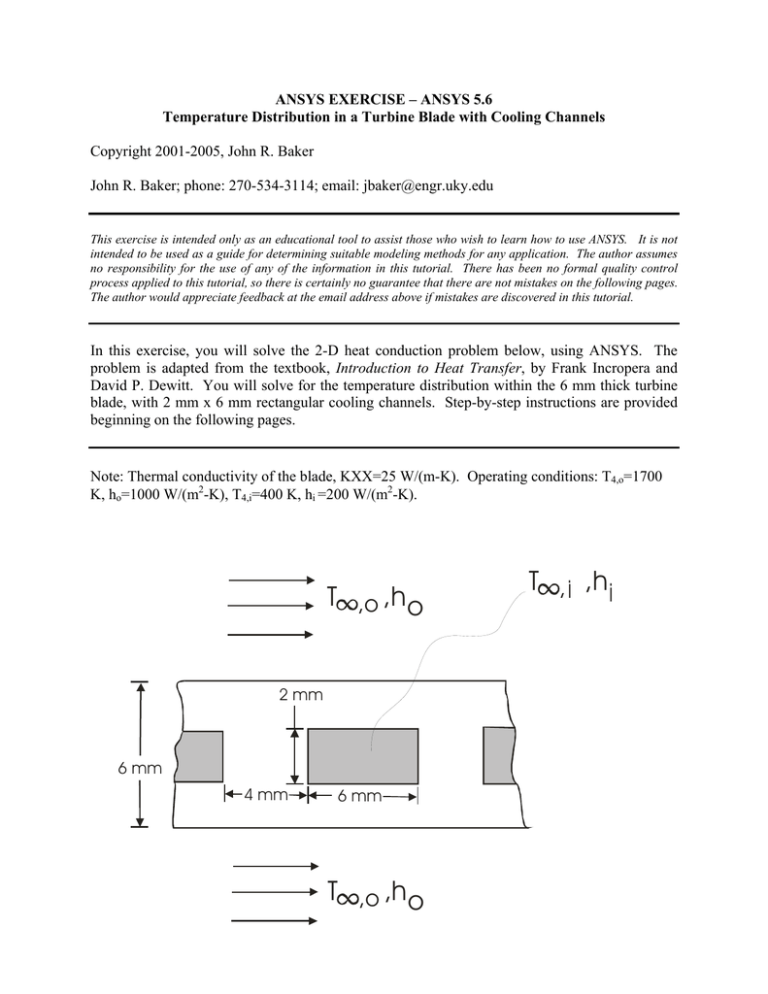
ANSYS EXERCISE – ANSYS 5.6
Temperature Distribution in a Turbine Blade with Cooling Channels
Copyright 2001-2005, John R. Baker
John R. Baker; phone: 270-534-3114; email: jbaker@engr.uky.edu
This exercise is intended only as an educational tool to assist those who wish to learn how to use ANSYS. It is not
intended to be used as a guide for determining suitable modeling methods for any application. The author assumes
no responsibility for the use of any of the information in this tutorial. There has been no formal quality control
process applied to this tutorial, so there is certainly no guarantee that there are not mistakes on the following pages.
The author would appreciate feedback at the email address above if mistakes are discovered in this tutorial.
In this exercise, you will solve the 2-D heat conduction problem below, using ANSYS. The
problem is adapted from the textbook, Introduction to Heat Transfer, by Frank Incropera and
David P. Dewitt. You will solve for the temperature distribution within the 6 mm thick turbine
blade, with 2 mm x 6 mm rectangular cooling channels. Step-by-step instructions are provided
beginning on the following pages.
Note: Thermal conductivity of the blade, KXX=25 W/(m-K). Operating conditions: T4,o=1700
K, ho=1000 W/(m2-K), T4,i=400 K, hi =200 W/(m2-K).
T ,o ,h o
2 mm
6 mm
4 mm
6 mm
T ,o ,h o
T , .I ,h.I
The steps that will be followed, after launching ANSYS, are:
Preprocessing:
1. Change Jobname.
2. Define element type. (Plane55 element, which is a 2-D, 4-node element for thermal analysis.)
3. Define material properties. (Thermal Conductivity -- only property required for this analysis.)
4. Create keypoints.
5. Create an area through keypoints.
6. Specify mesh density controls. (We will specify numbers of element divisions along lines.)
7. Mesh the area to create nodes and elements.
Solution:
8. Specify convection boundary conditions.
9. Specify zero heat flux through lines of symmetry.
10. Solve.
Postprocessing:
11. Plot the temperature distribution.
12. List locations of these center nodes by node number.
13. List the temperatures at each of these nodes.
Re-analysis
14. Modify Mesh / Re-analyze. (Primarily repeating earlier steps.).
Exit
15. Exit the ANSYS program, saving all data.
_____________________________________________________________________________
Launching ANSYS:
You should be able to simply click on the ANSYS icon on the Windows Desktop. The ANSYS
Launcher menu should appear. It is shown at the top of the next page. The only input you will
likely need on this menu is specification of your “Working Directory”. Specify any directory
(or, “Folder”) as your working directory. To browse to find the desired working directory, click
on the button with the three dots to the far right on the Launcher Menu on the line that says
“Working Directory”. Once the working directory is specified, click on “Run” at the bottom of
the Launcher Menu.
The ANSYS menus should open up. You will see a Main Menu, illustrated on the following
page, and a large black graphics window. You are now ready to begin creating the model and
performing the analysis.
ANSYS Launcher Menu:
ANSYS Main Menu:
Note: The menu picks needed to perform all required tasks are specified in italics in the stepby-step instructions below. It is sometimes more convenient to enter certain commands directly
at the command line. The command line is seen on the screen as:
The method of direct command line entry, however, is not covered in this exercise. Primarily, in
this exercise, the analysis will be performed using menu picks from the ANSYS Graphical User
Interface. Often, as an alternative, an input file, known as a “batch file”, is created, which is
simply an ASCII text file containing a string of ANSYS commands in the appropriate order.
ANSYS can read in this file as if it were a program, and perform the analysis in “batch mode”,
without ever opening up the Graphical User Interface. The batch file option is not covered in
this exercise.
SUGGESTION: As you work through this exercise, on the ANSYS Toolbar (upper right in the
ANSYS Graphical User Interface) click on “SAVE_DB” often! This Toolbar appears as:
At any point, if you want to resume from the previous time the model was saved, simply click on
“RESUM_DB” on this same Toolbar. Any information entered since the last save will be lost,
but this is a nice feature in the event that you make an input mistake, and are unsure of how to
correct it.
There are a number of ways to model a system and perform an analysis in ANSYS. The steps
shown on the following pages present only one method.
Preprocessing:
1. Change jobname. On the Utility Menu across the very top of the screen, select:
File -> Change Jobname
Enter “bladetmp”, and click on “OK”.
2. Define element type: Preprocessor -> Element Type -> Add/Edit/Delete
Click on “Add”. The “Library of Element Types” menu appears, as shown. Scroll down
to highlight “Thermal Solid”, and “Quad 4node 55” as shown. Click on “OK”, then
“Close”. Note that in ANSYS, this element is sometimes referred to as “Plane55”,
because it is a 2-D planar element, and it is element type 55 in the ANSYS element
library.
3. Define material properties: Preprocessor -> Material Properties -> -Constant- Isotropic
“OK” for material set number 1, then enter 25 for KXX (thermal conductivity), then click
on “OK”. KXX is the only material property needed for this analysis.
4. Create keypoints:
There are several options available for creating the basic geometry. The method that will
be employed involves creating “keypoints”, then generating an area, with corners defined
by the keypoints. Select:
Preprocessor -> -Modeling- Create -> Keypoints -> In Active CS…
Fill in the fields as shown at the top of the next page, then click “APPLY”. When you
click on “Apply”, the command is issued to create keypoint number 1 at (x,y,z)=(0.005,0.003,0). Note that when the Z field is left blank, in this case, the blank space
defaults to zero, which is desired. Since you clicked on “Apply”, instead of “OK”, then
the keypoint creation box remains open.
Create keypoint number 2 at (x,y,z)=(.005,.003,0), using the input shown below. After
entering the input, again, click on “APPLY”:
Create 6 total keypoints in the same manner. The locations for all 6 are shown in the
following table. When the final keypoint is created, click on “OK” instead of “APPLY”.
“OK” issues the command and also closes the keypoint creation box.
Keypoint Number
1
2
3
4
5
6
X-Location
-0.005
0
0
-0.003
-0.003
-0.005
Y-Location
0.003
0.003
0.001
0.001
0
0
Before moving on, it is probably a good idea to check the keypoint locations.
Along the top toolbar:
Choose: List -> Keypoints -> Coordinates Only. A box should open up with the
keypoint location information. If any keypoint is not in the correct location, at this point,
you can just re-issue the keypoint creation command for that particular keypoint. To do
this, choose: Preprocessor -> -Modeling- Create -> Keypoints -> In Active CS…
Fill in the correct information for that particular keypoint in the box, and click
“OK”. The keypoint will be moved to the correct location. If you have some keypoint
incorrectly numbered above number 6, this will not cause a problem. Just be sure you
have keypoint numbers 1 thru 6 located correctly.
You can close the box listing the keypoint locations, by clicking, in that listing
box, on “File-> Close”.
Note: In some cases, when you want to repeat the same process two or more times, you
can click “Apply” in the box, instead of “OK”. That issues the command, but leaves the
box open. Clicking “OK” issues the command, but leaves the box open. Sometimes,
though, using the “Apply” option can cause problems, if you are not careful. You might
click on “Apply” to issue the command, then immediately click on “OK” to close the
box, and this issues the command twice. Sometimes, that is not a problem, and
sometimes it is. So, in this exercise, in some cases below, you are just asked to click on
“OK” in each case, then repeat the entire procedure. You may instead choose to click on
“Apply”, if you are going to repeat the same process and you are confident this will not
cause problems. For the relatively simple remaining modeling effort in this exercise, the
approach of clicking “OK”, then re-opening the boxes does not add much work, and is
probably less likely to result in errors.
5. Create an area through keypoints.
This is a situation in which it is probably easiest to just enter the area creation
command at the command line. As shown below, enter the command: a,1,2,3,4,5,6
After typing in the command, hit “Enter”. A schematic (not to scale) of the area,
showing the corner keypoints, is also shown at the top of the next page.
1
2
4
6
3
5
6. Specify mesh density controls.
We will specify numbers of element divisions along lines. Choose:
Preprocessor -> -Meshing- Size Controls -> -Lines- Picked Lines
The picking menu (below left) appears. On the graphics window, click on the top
horizontal line (this is one with end keypoints 1 and 2), to highlight it. Then, click “OK”
in the picking menu. Then, the “Element Size” menu (below right) appears. Enter “5”
for “NDIV”, as shown, then click “OK”.
Now, repeat the above process to specify
• 2 divisions along the vertical line with end keypoints 2 and 3.
• 3 divisions along the horizontal line with end keypoints 3 and 4.
• 1 division along the vertical line with end keypoints 4 and 5.
• 2 divisions along the horizontal line with end keypoints 5 and 6.
• 3 divisions along the vertical line with end keypoints 6 and 1.
If you make a mistake on a particular line, just re-specify the divisions for a particular
line.
7. Mesh the rectangle to create nodes and elements:
Preprocessor -> -Meshing- Mesh -> Areas -> Free
A picking menu appears. Select “Pick All”. The area will be meshed. You will
see a number of small quadrilaterals drawn inside the area. Each small quadrilateral is a
“finite element”. There are four nodes associated with each individual element.
Solution:
8. Apply convection boundary conditions:
Solution -> -Loads- Apply -> -Thermal- Convection -> On Lines
A picking menu appears. Highlight the top horizontal line (with end keypoints 1
and 2), then click on “OK” in the picking menu. The box on the next page appears.
Enter “1000” for “Film Coefficient” and 1700 for “Bulk temperature”, as shown, and
click on “OK”. Repeat the process to apply the 200 W/(m2-K) film coefficient and the
400 K bulk temperature to the horizontal line, with end keypoints 3 and 4, and also to the
vertical line with end keypoints 4 and 5. This input is shown below.
9. Specify zero heat flux boundary conditions:
Solution -> -Loads- Apply -> -Thermal- Heat Flux -> On Lines
A picking menu appears. Highlight three lines: the line with end keypoints 1-6; the line
with end keypoints 2-3, and the line with end keypoints 5-6. When all three lines are
highlighted, just click “OK” in the picking menu, then in the box that subsequently
opens, just click “OK”. By default, this will specify a heat flux of zero along these three
lines, which is consistent with the symmetry of the problem.
10. Solve the problem: Solution -> -Solve- Current LS
Click “OK” in the “Solve Current Load Step” Box. Soon after clicking “OK”, you
should see a note in a yellow box saying “Solution is done!” You may close this yellow
box.
Postprocessing:
11. Plot the temperature distribution:
General Postproc -> Plot Results -> -Contour Plot- Nodal Solu
The box below appears. Highlight “DOF solution” and “Temperature TEMP”, as shown, and
click “OK”. In the graphics window, a plot, as shown at the bottom, should appear. This is a
temperature distribution color contour plot: Note that the temperature values corresponding to
the colors are shown in the legend to the right.
12. List the locations of the nodes.
On the top “Utility Menu”:
Choose List -> Nodes. In the green box that appears, just click on “OK” at the bottom.
A listing box appears showing the node locations. You can get a hard copy of the
information in this box by clicking, in this box: File -> Print. It should also be possible
to save this information to a file using the option, File -> Save As. However, this “Save
As” option does not appear to be working properly in the current ANSYS version.
13. List the temperatures at each of these nodes.
General Postproc -> List Results -> Nodal Solution
In the box that appears, highlight “DOF Solution” and “Temperature TEMP”, as shown,
then click “OK”.
A listing, as shown below, should appear. The locations of the same nodes have already
been listed, in Step 12 above, so the results for these nodes can be checked with the
textbook solution.
14. Modify Mesh / Re-analyze
The general idea in finite element modeling is that the finer the mesh (i.e. the more nodes
and elements used), the more accurate the solution. There is a cost associated with using
a large model, however. The solution time, the computer memory requirements, and the
computer hard drive space needed increase as the mesh density is increased. For this
particular analysis, however, unless an extremely fine mesh is used, the solution will
probably be completed very quickly, and the available memory and hard drive space
should be sufficient. This same problem can be re-solved, with a finer mesh, without
starting back at the beginning of these instructions. To do this, follow the steps below:
14a) Clear the existing nodes and elements:
Preprocessor -> -Meshing- Clear -> Areas
A picking menu appears. Select “Pick All”. At this point, the model in the graphics
window will probably disappear. However, the area still exists. You have only deleted
the nodes and elements. To see the area in the graphics window, you may need to click
on “Plot” on the top “Utility Menu”,
Then, choose “Areas”. The area should appear.
14b) Clear the previously specified mesh controls:
Preprocessor -> -Meshing- Size Controls -> -Lines- Clr Size
A picking menu appears. Select “Pick All”.
14c) Specify new mesh controls. Repeat step 6 from the initial analysis. Except, in this
case, use larger values for number of element divisions (NDIV).
14d) Remesh the model. Repeat step 7 from the initial analysis.
14e) Re-solve. Repeat step 10 from the initial analysis. You do not need to repeat steps
8 and 9 from the initial analysis. Specified boundary conditions s were applied to lines,
instead of directly to nodes. So, even though we re-meshed, the boundary conditions still
exist, because we never modified the lines that define the area.
14d) Post-process to obtain results for the finer mesh. Repeat steps 11-13 from the
previous analysis. For a finer mesh, you should see smoother curves on the temperature
contour plot.
15. Exit ANSYS, Saving All Data. On the ANSYS Toolbar, shown below, choose:
Quit ->Save Everything -> OK
To recall the model and solution at a later date, assuming you have deleted no files,
simply re-launch ANSYS, specify the same working directory as before, re-issue the
same jobname as used in Step 1 of these instructions, and then click on “RESUME_DB”
on the ANSYS Toolbar shown above.
To see the resumed model in the graphics window, you may then need to click on “Plot”
on the top “Utility Menu”,
Then, choose either “Elements”, “Nodes”, or “Areas”, depending on which entities you
wish to plot.