From: AAAI-93 Proceedings. Copyright © 1993, AAAI (www.aaai.org). All rights reserved.
Complexity
Analysis
of
Sven Koenig and Reid G. Simmons
School of C omputer Science
Carnegie Mellon University
Pittsburgh,
PA 15213-3891
skoenig@cs.cmu.edu,
reids@cs.cmu.edu
Abstract
This paper analyzes the complexity
of on-line reinforcement learning algorithms,
namely asynchronous
realtime versions of Q-learning and value-iteration,
applied
to the problem of reaching a goal state in deterministic
domains.
Previous work had concluded
that, in many
cases, tabula rasa reinforcement
learning was exponential for such problems, or was tractable only if the learning algorithm
was augmented.
We show that, to the
contrary, the algorithms
are tractable with only a simple change in the task representation
or initialization.
We provide tight bounds on the worst-case complexity,
and show how the complexity
is even smaller if the reinforcement
learning algorithms
have initial knowledge
of the topology
of the state space or the domain has
We also present a novel bicertain special properties.
directional
Q-learning
algorithm
to find optimal paths
from all states to a goal state and show that it is no
more complex than the other algorithms.
ntroduction
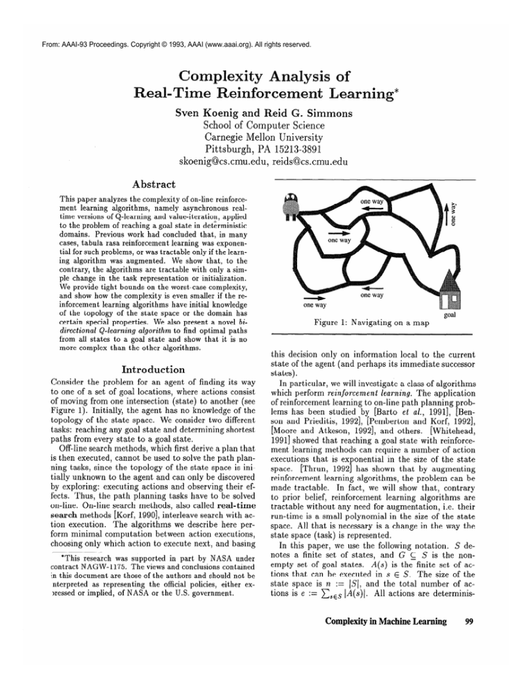
Consider the problem for an agent of finding its way
to one of a set of goal locations, where actions consist
of moving from one intersection (state) to another (see
Figure 1). Initially, the agent has no knowledge of the
topology of the state space. We consider two different
tasks: reaching any goal state and determining shortest
paths from every state to a goal state.
Off-line search methods, which first derive a plan that
is then executed, cannot be used to solve the path planning tasks, since the topology of the state space is initially unknown to the agent and can only be discovered
by exploring: executing actions and observing their effects. Thus, the path planning tasks have to be solved
on-line. On-line search methods, also called real-time
search methods [Korf, 19901, interleave search with action execution.
The algorithms we describe here perform minimal computation
between action executions,
choosing only which action to execute next, and basing
*This research was supported
in part by NASA under
contract NAGW-1175.
The views and conclusions
contained
in this document
are those of the authors and should not be
nterpreted
as representing
the official policies,
either exlressed or implied, of NASA or the U.S. government.
Figure 1: Navigating
on a map
this decision only on information local to the current
state of the agent (and perhaps its immediate successor
states).
In particular, we will investigate a class of algorithms
which perform reinforcement
learning. The application
of reinforcement learning to on-line path planning problems has been studied by [Barto et al., 19911, [Benson and Prieditis, 19921, [Pemberton and Korf, 19921,
[Moore and Atkeson, 19921, and others.
[Whitehead,
19911 showed that reaching a goal state with reinforcement learning methods can require a number of action
executions that is exponential in the size of the state
space.
[Thrun, 19921 h as shown that by augmenting
reinforcement learning algorithms, the problem can be
made tractable.
In fact, we will show that, contrary
to prior belief, reinforcement
learning algorithms are
tractable without any need for augmentation,
i.e. their
run-time is a small polynomial in the size of the state
space. All that is necessary is a change in the way the
state space (task) is represented.
In this paper, we use the following notation.
S denotes a finite set of states, and G C S is the nonempty set of goal states. A(s) is the finite set of actions that can be executed in s E S. The size of the
state space is n := ISI, and the total number of actions is e := xsES IA(s
All actions are determinis-
CompPexity in Machine Learn
tic. succ(s, a) is the uniquely determined successor state
when a E A(s) is executed in state s. The state space is
strongly connected, i.e. every state can be reached from
every other state. gd(s) denotes the goal distance of s,
i.e. the smallest number of action executions required
to reach a goal state from s. We assume that the state
space is totally observable’,
i.e. the agent can determine its current state with certainty, including whether
it is currently in a goal state.
Formally, the results of the paper are as follows. If a
good task representation or suitable initialization is chosen, the worst-case complexity of reaching a goal state
has a tight bound of O(n3) action executions for Qlearning and O(n2) action executions for value-iteration.
If the agent has initial knowledge of the topology of the
state space or the state space has additional properties,
the O(n3) bound can be decreased further. In addition,
we show that reinforcement
learning methods for finding shortest paths from every state to a goal state are
no more complex than reinforcement learning methods
that simply reach a goal state from a single state. This
demonstrates that one does not need to augment reinforcement learning algorithms to make them tractable.
Reinforcement
Learning
Reinforcement
learning is learning from (positive
and negative) rewards. Every action a E A(s) has an
immediate reward r(s, a) E R, that is obtained when
the agent executes the action.
If the agent starts in
s E S and executes actions for which it receives immediate reward rt at step t E No, then the total reward
that the agent receives over its lifetime for this particular behavior is
U(s):= 2 ytrt
t=Cl
where y E (0, l] is called the discount factor. If y < 1,
we say that discounting is used, otherwise no discounting is used.
Reinforcement
learning algorithms find a behavior
for the agent that maximizes the total reward for every possible start state. We analyze two reinforcement
learning algorithms that are widely used, namely Qlearning [Watkins, 19891 and value-iteration
[Bellman,
19571. One can interleave them with action execution
to construct asynchronous real-time forms that use actual state transitions rather than systematic or asynchronous sweeps over the state space. In the following,
we investigate these on-line versions: l-step Q-learning
and l-step value-iteration.
‘[Papadimitriou and Tsitsikhs, 19871 state results about
the worst-case complexity of every algorithm for cases where
the states are partially observable or unobservable.
100
Koenig
1. Set s := the current state.
2. If s E G, then stop.
3. Select an action a E A(s).
4. Execute action a.
/*
As a consequence,
the agent receives reward
r(s, a) and is in state SUCC(S,a). Increment the number of steps taken, i.e. set t := t + 1. */
5. Set Q(s, a) := r(.s, u) + yU(succ(3,
a)).
6. Go to 1.
where U(s) := max@=A(s) Q(s, a) at every point in time.
Figure 2: The (l-step)
Q-learning
algorithm
Q-Learning
The l-step Q-learning
algorithm2 [Whitehead,
19911
(Figure 2) stores information about the relative goodness of the actions in the states.
This is done by
maintaining a value Q(s, a) in state s for every action
a E A(s).
Q(s, a) approximates
the optimal total reward received if the agent starts in s, executes a, and
then behaves optimally.
The action selection step (line 3) implements the exploration rule (which state to go to next). It is allowed
to look only at information
local to the current state
The
s. This includes the Q-values for all a E A(s).
actual selection strategy is left open: It could, for example, select an action randomly, select the action that
it has executed the least number of times, or select the
action with the largest Q-value. Exploration is termed
undirected [Thrun, 19921 if it uses only the Q-values,
otherwise it is termed directed.
After the action execution step (line 4) has executed
the selected action a, the value update step (line 5)
adjusts Q(s, a) (and, if needed, other information
local to the former state). The l-step look-ahead value
T(S, a)+yU(succ(s,
a)) is more accurate than, and therefore replaces, &(s, a).
Value-Iteration
The l-step value-iteration
algorithm is similar to the
l-step Q-learning algorithm. The difference is that the
action selection step can access T(S, a) and U(succ(s, a))
for every action a E A(s) in the current state s,
whereas Q-learning has to estimate them with the Qvalues. The value update step becomes “Set U(s) :=
maxaEqs)(r(s,
a) + yu(succ(s,
a)))“.
Whereas Q-learning does not know the effect of an
action before it has executed it at least once, valueiteration only needs to enter a state at least once to
discover all of its successor states. Since value-iteration
is more powerful than Q-learning, we expect it to have
a smaller complexity.
2Since the actions have deterministic outcomes, we state
the Q-learning algorithm with the learning rate cv set to one.
Task Representation
To represent the task of finding shortest paths as a reinforcement learning problem, we have to specify the
reward function r. We let the lifetime of the agent in
formula (1) en d w h en it reaches a goal state. Then, the
only constraint on T is that it must guarantee that a
state with a smaller goal distance has a larger optimal
total reward and vice versa. We consider two possible
reward functions with this property.
In the goal-reward
representation,
the agent is
rewarded for entering a goal state, but not rewarded
This representation
has been
or penalized otherwise.
used by [Whitehead,
19911, [Thrun, 19921, [Peng and
Williams, 19921, and [Sutton, 19901, among others.
r(s,a)
1
0
=
if succ(s, a) E G
otherwise
The optimal total discounted reward of s E S - G :=
{s E S : s e 6) is y gd(s)-l.
If no discounting is used,
then the optimal total reward is 1 for every s E S - G,
independent of its goal distance.
Thus, discounting is
necessary so that larger optimal total rewards equate
with shorter goal distances.
representation,
the agent is
In the action-penalty
penalized for every action that it executes, i.e. T(S, a) =
-1. This representation has a more dense reward structure than the goal-reward representation (i.e. the agent
receives non-zero rewards more often) if goals are relatively sparse. It has been used by [Barto et al., 19891,
[Barto et ad., 19911, and [Koenig, 19911, among others.
The optimal total discounted reward of s E S is (1 Ygdcs) >/(y - 1). Its optimal total undiscounted reward
is -gd(s).
Note that discounting can be used with the
action-penalty
representation,
but is not necessary.
Compiexit-y
of
caching a Goal State
We can now analyze the complexity
of reinforcement
learning algorithms for the path planning tasks. We
first analyze the complexity of reaching a goal state for
the first time.
The worst-case complexity
of reaching a goal state
with reinforcement
learning (and stopping there) provides a lower bound on the complexity
of finding abb
shortest paths, since this cannot be done without knowing where the goal states are. By “worst case” we mean
an upper bound on the total number of steps for a tabula rasa (initially uninformed)
algorithm that holds for
all possible topologies of the state space, start and goal
states, and tie-breaking rules among actions that have
the same Q-values.
Assume
that
a Q-learning
algorithm
is zeroinitialized (all Q-values are zero initially) and operates
on the goal-reward representation.
Note that the first
Q-value that changes is the Q-value of the action that
leads the agent to a goal state. For all other actions,
no information about the topology of the state space is
remembered and all Q-values remain zero. Since the action selection step has no information on which to base
its decision if it performs undirected exploration,
the
agent has to choose actions according to a uniform distribution and thus performs a random walk. Then, the
agent reaches a goal state eventually, but the average
number of steps required can be exponential in n, the
number of states [Whitehead, 19911.
This observation motivated [Whitehead, 19911 to explore cooperative reinforcement learning algorithms in
order to decrease the worst-case complexity.
[Thrun,
19921 showed that even non-cooperative
algorithms
have polynomial worst-case complexity if reinforcement
learning is augmented with a directed exploration mechanism (“counter-based
Q-learning”).
We will show that
one does not need to augment Q-learning: it is tractable
if one uses either the action-penalty
representation
or
different initial Q-values.
Using
a Different
Task
Representation
Assume we are still using a zero-initialized
Q-learning
algorithm, but let it now operate on the action-penalty
representation.
Although the algorithm is still tabula
rasa, the Q-values change immediately,
starting with
the first action execution, since the reward structure
is dense. In this way, the agent remembers the effects
of previous action executions.
We address the case in
which no discounting is used, but the theorems can easily be adapted to the discounted case. [Koenig and Simmons, 19921 contains the proofs, additional theoretical
and empirical results, and examples.
Definition 1 Q-values are culled consistent in, for uld
s E G and a E A(s), Q(s, a) = 0, and, for all s E S - G
and a E A(s), -1 + U(succ(s, a)) 5 Q(s, a) 5 0.
Definition 2 An
undiscounted
Q-learning
algorithm with action-penalty
representation
is culled
admissible3 iff its initial Q-values are consistent and
its action selection step is “a := urgmux,,EA~s~Q(s,
a’) “.
If a Q-learning algorithm is admissible, then its Qvalues remain consistent and are monotonically
decreasing.
Lemma 1 contains the central invariant for all
proofs. It states that the number of steps executed so
far is always bounded by an expression that depends
only on the initial and current Q-values and, more over,
“that the sum of all Q-values decreases (on average)
by one for every step taken” (this paraphrase is grossly
simplified). A time superscript of t in Lemmas 1 and 2
refers to the values of the variables immediately before
executing the action during step t.
Lemma
1 For all steps t E J’& (until termination)
of
an undiscounted,
admissible Q-learning algorithm with
31f the value update step is changed to “Set Q(s, a) :=
min(Q(s,
a), -1 +yU(succ(s,
a)))“, then the initial Q-values
need only to satisfy that, for all s E G and a E A(s),
Q(s,u)
= 0, and, for all s E S - G and a E A(s),
-1 - gd(szlcc(s,u))
2 Q(s, a) < 0. Note that Q(s, a) =
-1 - h(succ(s,
u)) h as this property, where h is an admissible heuristic for the goal distance.
action-penalty
representation,
Ut(st)
+c x
Q”(s, a) - t 2
sES aEA(s)
c c Qt(s,
a)+ U"(so)
-loopt
sES 64(s)
and
Figure 3: A worst-case
example
goal
coopt
5 &S C~EA(S)(~~(S,
u>
- Qtbu))j
where doopt := I{t’ E (0,. . . , t - 1) : st’ = s”+~}] (the
number of actions executed before t that do not change
the state).
Lemma 2 An undiscounted,
admissible Q-learning adgorithm with action-pen&y
representation
reaches a
goal state and terminates
after at most
2
x
SES-G
c
aEA(s)
(Q’(s, a) + gd(succ(s,
a)) + 1) - u”bo)
steps.
Theorem
1 An admissible Q-learning algorithm with
action-pen ulty representation
reaches a goal state and
terminates
after at most O(en) steps.
Lemma 2 utilizes the invariant and the fact that each
of the e different Q-values is bounded by an expression that depends only on the goal distances to derive a bound on t. Since the sum of the Q-values decreases with every step, but is bounded from below, the
algorithm must terminate.
Because the shortest distance between any two different states (in a strongly
connected graph) is bounded by n - 1, the result of
Theorem 1 follows directly.
Note that Lemma 2 also
shows how prior knowledge of the topology of the state
space (in form of suitable initial Q-values) makes the
Q-learning algorithm better informed and decreases its
run-time.
If a state space has no duplicate actions, then e 5 n2
and the worst-case complexity
becomes O(n3).
This
provides an upper bound on the complexity of the Qlearning algorithm . To demonstrate
that this bound
is tight for a zero-initialized
Q-learning algorithm, we
show that O(n3) is also a lower bound: Figure 3 shows
a state space where at least 1/6n3 - 1/6n steps may
be needed to reach the goal state. To summarize, although Q-learning performs undirected exploration, its
worst-case complexity
is polynomial
in n. Note that
Figure 3 also shows that every algorithm that does not
know the effect of an action before it has executed it at
least once has the same big-0 worst-case complexity as
zero-initialized
Q-learning.
Using
Different
Initial
&-values
We now analyze Q-learning algorithms that operate on
the goal-reward representation,
but where all Q-values
are initially set to one. A similar initialization has been
used before in experiments
conducted
by [Kaelbling,
19901.
102
Koenig
If the action selection strategy is to execute the action with the largest Q-value, then a discounted, oneinitialized Q-learning algorithm with goal-reward representation behaves identically to a zero-initialized
Qlearning algorithm with action-penalty
representation
if all ties are broken in the same way.4 Thus, the complexity result of the previous section applies and a discounted, one-initialized Q-learning algorithm with goalreward representation reaches a goal state and terminates after at most O(en) steps.
Gridworlds
We have seen that we can decrease the complexity
of
Q-learning dramatically
by choosing a good task representation or suitable initial Q-values. Many domains
studied in the context of reinforcement
learning have
additional properties that can decrease the worst-case
complexity
even further.
For example, a state space
topology has a linear upper action bound b E No iff
e 5 bn for all n E NO. Then, the worst case complexity
becomes O(bn2) = O(n2).
Gridworlds, which have often been used in studyin
reinforcement learning [Barto et ad., 19891 [Sutton, 1990!i
[Peng and Williams, 19921 [Thrun, 19921 have this property. Therefore, exploration in unknown gridworlds actually has very low complexity.
Gridworlds often have
another special property. A state space is called l-step
invertible [Whitehead, 19911 iff it has no duplicate actions and, for all s E S and a E A(s), there exists an
a’ E A(succ(s, a)) such that s~cc(s~cc(s,
a), a’) = s.
(We do not assume that the agent knows that the state
space is l-step invertible.)
Even a zero-initialized
Qlearning algorithm with goal-reward representation (i.e.
a random walk) is tractable for l-step invertible state
spaces, as the following theorem states.
Theorem 2 A zero-initialized
Q-learning
udgorithm
with goal-reward representation
reaches a goad state and
terminates in at most O(en) steps on average ifthe state
space is l-step invertible.
This theorem is an immediate corollary to [Aleliunas
et al., 19791. If the state space has no duplicate actions,
4This is true only for the task of reaching a goal state.
In general, a discounted,
“one-initialized”
Q-learning
algorithm with goal-reward
representation
behaves identically
to a “(minus
one)-initialized”
Q-learning
algorithm
with
action-penalty
representation
if in both cases the Q-values
of actions in goal states are initialized to zero.
Initially,
Qr(s,a)
= Qb(s, a)
for all s E S and a E A(s).
1. Set s := the current
2. Ifs
0 and
done(s,a)
=
f&e
state.
E G, then set done(s,a)
3. If done(s)
4.
=
:= trzde for all a E A(s).
= trzse, then go to 8.
/* forward step */
Set a := argmax,,EA(sjQf(s,
a’).
the agent re5. Execute action a. (As a consequence,
ceives reward -1 and is in state succ(s,u).)
SUCC(S, a)) and done(s,
6. Set Qf(s, a) := -l+Uf(
done(succ(s,
u)).
a) :=
7. Go to 1.
8. /* backward step */
Set a := argmax,,CAC,~Qb(s,
a’).
the agent re9. Execute action a. (As a consequence,
ceives reward -1 and is in state succ(s,u).)
10.
set
Qb(s,
U)
:=
11. If ub(S) 5 -n,
12.
-1
i- ub(suCC(S,
U)).
then stop.
Go to 1.
where, at every point in time,
Uj(S) := ma&EA(
s) Q.f by a>,
&(s)
:=
done(s)
m%EA(
:=
s) Qb(%
3,,~(,>(Qf(s,
a>>
a)
and
=
Figure 4: The bi-directional
uf(s)
A done@,
a>>.
Q-learning
algorithm
then the worst-case complexity
becomes O(n3).
This
bound is tight. Thus, the average-case complexity of a
random walk in l-step invertible state spaces is polynomial (and no longer exponential)
in n. For l-step
invertible state spaces, however, there are tabula rasa
on-line algorithms that have a smaller big-0 worst-case
complexity than Q-learning [Deng and Papadimitriou,
19901.
eterrnining
Optimal
olicies
We now consider the problem of finding shortest paths
from udl states to a goal state.
We present a novel
extension
of the
Q-learning
algorithm
that
determines
the goal distance of every state and has the same big0 worst-case complexity as the algorithm for finding a
single path to a goal state. This produces an optimal
deterministic
policy in which the optimal behavior is
obtained by always executing the action that decreases
the goal distance.
The algorithm, which we term the bi-directional
$learning algorithm,
is presented in Figure 4. While
the complexity results presented here are for the undiscounted,
zero-initialized
version with action-penalty
representation,
we have derived similar results for all
of the previously described alternatives.
The bi-directional
Q-learning algorithm iterates over
two independent Q-learning searches: a forward phase
that uses &f-values to search a state s with done(s) =
true from a state s’ with done(s’)
= false, followed
by a backward phase that uses Qb-values to search
a state s with done(s)
= false from a state s’ with
done(s’) = true. The forward and backward phases are
implemented using the Q-learning algorithm from Figure 2.
The variables done(s) h ave the following semantics: If
done(s) = true, then Uf(s) = -gd(s)
(but not necessarily the other way around).
Similarly for the variables
done(s, a) for s E S - G: If done(s,a)
= true, then
Qf(s, a) = -1 - gd(succ(s, a)).
If the agent executes a in s and done(succ(s,
a)) =
true, then it can set done(s, a) to true. Every forward
phase sets at least one additional done(s, a) value to
true and then transfers control to the backward phase,
which continues until a state s with done(s)
= false
is reached, so that the next forward phase can start.
After at most e forward phases, done(s) = true for all
s E S. Then, the backward phase can no longer find a
state s with done(s) = f a 1se and decreases the Ub-values
beyond every limit. When a Ub-value reaches or drops
below -n, the agent can infer that an optimal policy
has been found and may terminate.
See [Koenig and
Simmons, 19921 for a longer description and a similar
algorithm that does not need to know n in advance,
always terminates no later than the algorithm stated
here, and usually terminates shortly after done(s)
=
true for all s E S.
Theorem 3 The bi-directional
&-learning
algorithm
finds an optimal policy and terminates
after at most
0( en) steps.
The proof of Theorem 3 is similar to that of Theorem 1. The theorem states that the bi-directional
Qlearning algorithm has exactly the same big-0 worstcase complexity as the Q-learning algorithm for finding
a path to a goal state. The complexity becomes O(n3)
if the state space has no duplicate actions.5 That this
bound is tight follows from Figure 3, since determining
an optimal policy cannot be easier than reaching a goal
state for the first time. It is surprising, however, that
the big-0 worst-case complexities for both tasks are the
same.
Figures 5 and 6 show the run-times of various reinforcement learning algorithms in reset state spaces (i.e. state
spaces in which all states have an action that leads back
to the start state) and one-dimensional
gridworlds of
sizes n E [2,50], in both cases averaged over 5000 runs.
The x-axes show the complexity of the state space
(measured as en) and the y-axes the number of steps
needed to complete the tasks. We use zero-initialized
algorithms with action-penalty
representation, with ties
broken randomly. For determining optimal policies, we
distinguish two performance measures: the number of
steps until an optimal policy is found (i.e. until U(s) =
5The bi-directional
Q-learning
algorithm
can be made
more efficient, for example by breaking ties intelligently,
but
this does not change its big-0 worst-case complexity.
Complexity in Machine Learning
183
goal
goal
Reset
State
Space
2500
0
Figure 5: Reset state space
-gd(s)
for every state s), and the number of steps unti I
the algorithm realizes that and terminates.
These graphs confirm our expectation about the var
ious algorithms.
For each algorithm,
Q-learning and
value-iteration ++expect
its run-time (i.e. number of
steps needed) for reaching a goal state to be smaller
than the run-time for finding an optimal policy which
we expect, in turn, to be smaller than the run-time for
terminating with an optimal policy. We also expect the
run-time of the efficient? value-iteration
algorithm to
be smaller than the run-time of the efficient Q-learning
algorithm which we expect to be smaller than the runtime of a random walk, given the same task to be solved.
In addition to these relationships, the graphs show that
random walks are inefficient in reset state spaces (where
they need 3 x 2n-2 - 2 steps on average to reach a
goal state), but perform much better in one-dimensional
gridworlds (where they only need (n- 1)2 steps on average), since the latter are l-step invertible. But even for
gridworlds, the efficient Q-learning algorithms continue
to perform better than random walks, since only the
former algorithms immediately
remember information
about the topology of the state space.
Extensions
The complexities
presented here can also be stated in
terms of e and the depth of the state space d (instead
of n), allowing one to take advantage of the fact that
104
Koenig
1000
1400
2000
2500
Figure 6: One-dimensional
2500
en
6 “Efficient” means to use either the action-penalty
resentation or one-initialized Q-values (U-values).
500
rep-
3000
3500
4000
4500
gridworld
the depth often grows sublinearly in n. The depth of a
state space is the maximum over all pairs of different
states of the length of the shortest path between them.
All of our results can easily be extended to cases where
the actions do not have the same reward. The result
about l-step invertible state spaces also holds for the
more general case of state spaces that have the following
property: for every state, the number of actions entering
the state equals the number of actions leaving it.
Reinforcement
learning algorithms
can be used in
state spaces with probabilistic
action outcomes.
Although the results presented here provide guidance for
modeling probabilistic
domains, more research is required to transfer the results.
[Koenig and Simmons,
19921 contains a discussion of additional challenges encountered in probabilistic
domains.
Conclusion
Many real-world domains have the characteristic of the
task presented here - the agent must reach one of a
number of goal states by taking actions, but the initial
topology of the state space is unknown.
Prior results
which indicated that reinforcement learning algorithms
were exponential in n, the size of the state space, seemed
to limit their usefulness for such tasks.
This paper has shown, however, that such algorithms
are tractable when using either the appropriate task representation or suitable initial Q-values.
Both changes
produce a dense reward structure,
which facilitates
learning.
In particular,
we showed that the task of
reaching a goal state for the first time is reduced from
exponential to O(en), or O(n3) if there are no duplicate
actions. Furthermore, the complexity is further reduced
if the domain has additional properties, such as a linear
Tight bounds on the number of steps required in the worst
case for reaching a goal state using a zero-initialized
algorithm with action-penalty
representation
or a one-initialized
algorithm with goal-reward
representation;
the same results
apply to determining
optimal policies
State
Q-Learning
Space
general case
no duplicate
linear upper
actions
action bound
Figure 7: Complexities
Value-Iteration
ok4
O(n3)
O(n2)
m2>
Ob2)
O(n2)
of Reinforcement
Learning
95, Department
of Computer
sachusetts at Amherst.
Acknowledgements
Avrim Blum, Long-Ji Lin, Michael Littman, Joseph
O’Sullivan, Martha Pollack, Sebastian Thrun, and especially Lonnie Chrisman (who also commented on the
proofs) provided helpful comments on the ideas presented in this paper.
eferences
Aleliunas,
R.; Karp, R.M.; Lipton,
R. J.; Loviisz, L.; and
Rackoff,
C. 1979.
Random
walks, universal traversal sequences,
and the complexity
of maze problems.
In 20th
Annual
Symposium
on Foundation
of Computer
Science,
San Juan, Puerto Rico. 218-223.
Barto, A.G.; Sutton, R.S.; and Watkins, C.J. 1989. Learning and sequential decision making. Technical
Report 89-
University
of Mas-
Barto, A.G.; Bradtke, S.J.; and Singh, S.P. 1991. Real-time
learning and control using asynchronous
dynamic programming. Technical
Report 91-57, Department
of Computer
Science, University of Massachusetts
at Amherst.
Bellman, R. 1 957. Dynamic
versity Press, Princeton.
Programming.
Princeton
Uni-
Benson, G.D. and Prieditis, A. 1992. Learning continuousspace navigation
heuristics
in real-time.
In Proceedings
of the Second International
Conference
on Simulation
of
Adaptive
Behavior:
From Animals
to Animats.
Deng, X. and Papadimitriou,
known graph. In Proceedings
upper action bound.
In l-step invertible state spaces,
even the original, inefficient algorithms have a polynomial average-case complexity.
We have introduced
the novel bi-directional
Qlearning algorithm for finding shortest paths from all
states to a goal and have shown, somewhat surprisingly,
that its complexity is O(en) as well. This provides an
efficient algorithm to learn optimal policies. While not
all reinforcement learning tasks can be reformulated as
shortest path problems, the theorems still provide guidance: the run-times can be improved by making the reward structure dense, for instance, by subtracting some
constant from all immediate rewards.
The results derived for Q-learning can be transferred
to value-iteration
[Koenig, 19921 [Koenig and Simmons,
19921. The important results are summarized in Figure 7. Note that a value-iteration
algorithm that always executes the action that leads to the state with
the largest U-value is equivalent to the LRTA* algorithm [Korf, 19901 with a search horizon of one if the
state space is deterministic and action penalty representation is used [Barto et a!., 19911.
In summary, reinforcement
learning algorithms are
useful for enabling agents to explore unknown state
spaces and learn information
relevant to performing
tasks. The results in this paper add to that research
by showing that reinforcement learning is tractable, and
therefore can scale up to handle real-world problems.
Science,
C.H. 1990. Exploring
of the FOCS.
an un-
Kaelbling,
L.P. 1990.
Learning
in Embedded
Systems.
Ph.D. Dissertation,
Computer
Science Department,
Stanford University.
Koenig, S. and Simmons,
R.G. 1992. Complexity
analysis of real-time reinforcement
learning applied to finding
shortest paths in deterministic
domains.
Technical
Report
CMU-CS-93-106,
School of Computer
Science, Carnegie
Mellon University.
Koenig,
S. 1991.
Optimal
probabilistic
and decisiontheoretic planning using M arkovian decision theory. M aster’s thesis, Computer
Science Department,
University
of
California
at Berkeley.
(Available
as Technical
Report
UCB/CSD
92/685).
Koenig, S. 1992. The complexity
of real-time search. Technical Report CMU-CS-92-145,
School of Computer
Science, Carnegie Mellon University.
Korf, R.E. 1990. Real-time
telligence
42(2-3):189-211.
heuristic
search.
Artificial
In-
Moore, A.W. and Atkeson, C.G. 1992. Memory-based
reinforcement learning: Efficient computation
with prioritized
sweeping. In Proceedings
of the NIPS.
Papadimitriou,
C.H. and Tsitsiklis,
J.N. 1987. The complexity of Markov decision processes.
Mathematics
of Op12(3):441-450.
erations
Research
Pemberton,
J.C. and Korf, R.E. 1992. Incremental
path
planning on graphs with cycles. In Proceedings
of the First
Annual
AI Planning
Systems
Conference.
179-188.
R.J. 1992. Efficient learning and
Peng, J. and Williams,
planning within the Dyna framework.
In Proceedings
of the
Second International
Conference
on Simulation
of Adaptive
Behavior:
From Animals
to Animats.
Sutton, R.S. 1990. Integrated
architectures
for learning,
planning,
and reacting based on approximating
dynamic
programming.
In Proceedings
of the Seventh
International
Conference
on Machine
Learning.
The role of exploration
in learning
Thrun,
S.B. 1992.
control
with neural networks.
In White,
David A. and
Sofge, Donald A., editors
1992, Handbook
of Intelligent
Control:
Neural, Fuzzy and Adaptive
Approaches.
Van Nostrand Reinhold, Florence, Kentucky.
Watkins, C. J. 1989. Learning
Dissertation,
King’s College,
from Delayed Rewards.
Cambridge
University.
Ph.D.
Whitehead,
S.D. 1991. A complexity
analysis of cooperative mechanisms
in reinforcement
learning.
In Proceedings
of the AAAI.
607-613.
Complexity in Machine Leaming
105