From: AAAI-86 Proceedings. Copyright ©1986, AAAI (www.aaai.org). All rights reserved.
NOISETOLERANT
RANGE ANALYSIS
FOR AUTONOMOUS NAVIGATION
l
Aviv Bergman and Cregg K. Cowan
Robotics Laboratory, SRI International
333 Ravenswood Avenue, Menlo Park, California
ABSTRACT
Techniques for detecting horizontal
regions,
obstacles, ditches, and shoulders along a road from
range data are described. The noise level in each scan
line of the range image is computed and an adaptive
threshold is used for noise compensation. The sources of
noise and the scanning geometry for a time-of-flight
range sensor are discussed and experimental results of
applying these techniques to ERIM range images are
presented.
I
II
94025
DESCRIPTION
OF RANGE IMAGERY
In this section we describe characteristics of range
sensors that use the phase difference between the reference and reflected signals of a modulated laser beam to
determine the range to a surface [I]. See [3] and [4] for
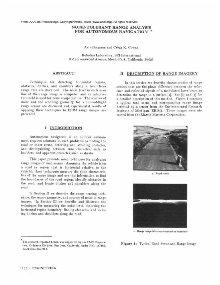
a detailed description of this method. Figure 1 contains
a typical road scene and corresponding range image
detected by a sensor from the Environmental Research
Institute of Michigan (ERIM). These images were obtained from the Martin Marietta Corporation.
INTRODUCTION
Autonomous navigation in an outdoor environment requires solutions to such problems as finding the
road or other route, detecting and avoiding obstacles,
and distinguishing between true obstacles, such as
boulders, and apparent obstacles, such as shrubs.
This paper presents some techniques for analyzing
range images of road scenes. Assuming the vehicle is on
a road (a region that is horizontal relative to the
vehicle), these techniques measure the noise characteristics of the range image and use this information to find
the boundaries of the road region, identify obstacles in
the road, and locate ditches and shoulders along the
road.
a.
Road scene
In Section II we describe the range sensing technique, the sensor geometry, and sources of noise in range
images. In Section III we describe and illustrate the
techniques for measuring the noise level, detecting the
horizontal region boundary, finding obstacles, and locating ditches and shoulders along the road.
b. Range image
*
The research reported herein was supported by the FMC Corporation, Ordnance Division, San Jose, California, under P.O. 147466,
Work Directive 014.
1122 / ENGINEERING
(distance
encoded
as intensity)
Figure 1: Typical Road Scene and Range Image
Because the ERIM sensor uses the phase difference
between two signals to measure distance, the range
values obtained are inherently ambiguous--objects
whose
distance from the sensor differs by exactly one modulation cycle have the same range value. For the ERIM
sensor, the distance corresponding
to one modulation
cycle (the ambiguity interval) is 64 feet.
A.
b
r
P
x”“4\,
ScanninE Geometry
The configuration
for sensing the range r to a
world point P is illustrated in Figure 2. In this diagram
the sensor lies on the z axis with its principal ray in the
x-z plane. The tilt of the sensor is given by angle $,
and ,8 is the pan angle from the center of the scan line.
An ERIM range image consists of 64 horizontal scan
lines, and each scan line contains 256 range values
(obtained by sweeping the laser from -/3,,, to +Pmax).
B.
!J
P
Figure 2: Sensor Geometry:
Range r, Tilt +
and Pan @
Sources of Noise in Range Images
----
Two noise effects of particular
interest for an
autonomous
vehicle operating in an outdoor environment are absorption and scattering of the laser beam by
the atmosphere and noise contributed
by background
radiation, such as sunlight. Other noise sources for a
laser ranging device are described in (51.
The transmission loss from atmospheric effects is
dependent on the range to the object surface and on the
wavelength of the laser. For the ERIM sensor, the principal transmission
loss is due to scattering [5! and is
proportional to cmkB, where r is the range to the surface
and k is a constant dependent on the laser wavelength
and the visibility.
The detected signal strength
surface orientation and reflectivity.
received signal is of the form
Scan
P(pf(
-y
x (l-
also depends on the
Therefore the total
c+)
where PO is the transmitted
power, p is the diffuse surface reflectance, 19 is the angle between the incident
beam and the surface normal, and r is the range.
Figure 3 shows the scanning configuration for the
ERIM road images.
The relative angle between the
road surface and the laser becomes more oblique for
higher scan lines.
Although
the received
signal
decreases for higher scan lines (cos 0 decreases and r
increases), the ERIM device has constant integration
time for each range value, resulting in decreased signal
to noise ratio for higher scan lines. (Other devices vary
the integration time to achieve a constant signal to noise
ratio (41).
63
0
Figure 3: Configuration for Scanning
(Side View)
III
A.
p CO80
line
.. -
a Road
RANGE IMAGE ANALYSIS
Correcting for Range Ambiguity
The first step in analyzing a range image is to
remove the ambiguity interval. We analyze each column
in the image starting from the bottom; if we detect a
decrease in range value greater than a threshold
(currently 16 feet), we assume it to bei caused by the
ambiguity interval and add 64 feet to the measured
range value.
This simple technique fails for some cases where
the laser spot spans a range discontinuity
(part of the
spot is on the close object and part on the more distant
object).
In such cases the measured range value is an
average of the range to the two surfaces. If the surfaces
lie in different ambiguity intervals, then the measured
range value can produce an arbitrarily small decrease in
range, falling below the threshold.
We correct such
cases by hand.
A method for automatically
removing
the ambiguity interval is described in [2].
VISION
AND SIGNAL
UNDERSTANDING
/
1123
B.
Measuring --the Noise Level
Although some sources of range data noise can be
modeled a priori, other noise sources, such as the orientation and reflectivity of the target surface, are not
generally known. We therefore choose to estimate the
total noise by measuring the statistical characteristics of
the actual range data. We currently measure the mean
~1and standard deviation o for each scan line.
Consider the values for one scan line when viewing
a horizontal plane (the x-y plane) that is aligned with
the range sensor as shown in Figure 4a. The range sensor lies on the z axis with its principal ray in the x-z
plane. The line P,P, is the intersection of the x-y plane
with
the scanning plane (formed by sweeping from
The range value r for an arbitrary
-4nax to +p,,).
point P is related to the range value along the principal
ray r. by b = rO / co9 p]. Figure 4b displays this
relationship
a. Sensor geometry
between range and pan angle.
Range
Under the assumption that the horizontal plane is
aligned with the sensor, that is, that the vehicle is not
tilted relative to the road surface, the maximum range
difference between the center and edge of each scan line
is (ru - rO /cos(p,,)).
If we multiply each value by
cos /3 to compensate for its pan angle, then the range
values within the horizontal region become constant.
Measuring the mean ~1 and standard deviation Q of the
modified range values for each scan line can then be
considered as local estimation of the noise parameters p
and u for the range image.
Because we do not expect the horizontal region to
fill the entire image, we measure p and o only in an
“adaptive” analysis window of each scan line. This window is based on the boundary of the horizontal region
detected in the previous scan line. The analysis window
for the first scan line is the entire line (the first scan line
is assumed to be entirely in the road).
In order to
eliminate the effect of obstacles or ditches when measuring 0, we include only those points in the value range
p f k/r. Another technique to eliminate the effect of
obstacles on the standard deviation of the ith scan line
(gi) is to discard those points with value outside
pi f
kai 1 (based on the assumption that the noise
The following sections describe
level changes slowly).
the use of p and 0 in detecting the horizontal region
boundaries and finding obstacles in the region.
1124
/ ENGINEERING
I
1
I
I
I
4 max
0
P max
Pan angle
b. Range vs. pan angle
Figure 4: Scanning
C.
a Horizontal
Plane
Detecting Horizontal Region Boundaries
Given
pi and bi, we detect
the left road-region
boundary of the ith scan line by locating a sequence of
range values that are within p f k,a. We start searching for this sequence at a point k, pixels outsidl:, (to the
left of) the left boundary of the previous scan line. The
parameter k, is currently set to zero because of perspective; we expect the apprarent
road width to narrow
slowly with increasing distance.
The left boundary is
the first point in the sequence. We limit the change in
boundary position to a value based on the width of the
road detected in the previous scan line in order to
safeguard later processing from possible errors. Detecting the right boundary is similar.
An example of this processing is shown in
Figure 5. The lower-left corner displays an ERIM image that has been correctedfor ambiguity interval. The
lower-right corner plots range values for several scan
lines and illustrates the characteristic curvature of
horizontal regions (compare to Figure 4b). Note the
large changein range values along two scan lines that is
causedby the presenceof an obstacle.The upper right
shows plots of range values after correcting for the pan
angle. The location of the road boundaries are also
marked in the upper right. The upper-left corner displays the detectedroad region. The arrow in the upperleft corner indicates the range image rows that contain
the obstacle.
Figure
6: Detecting Jump Boundaries
We found that using d to detect jump boundaries
provides better results than other methods that we
tested. Figure 7 showsjumps detectedwhen
d’>k
(r = range value) .
This dynamic thrresholdmethod correctly locatesdistant
obstacles and does not miss significant range discontinuities near the vehicle. However,this techniqueis adversely affectedby the noise at the bottom of the image.
Figure
1).
6: Detecting the Road Region
Detecting
Jump Boundaries
Using Sigma
After locating the left and right road boundaries
and calculating ~1and u, we detect obstaclesby finding
horizontal and vertical discontinuities in range values
(called jump boundaries)as specifiedbelow. The value
ri 9j is the range value for pixel j on scan line i.
l
Smooth the range values between the
left and right road boundariesusing a 1
by 3 kernel.
l
l
Detect a horizontal jump if
I > ‘lai’
I ‘i 9 Detect a vertical jump if
I ‘i I > c2bkl’
,
j
'i,j+Q
j
'Cl,j
After detecting thesejump boundary locations,we
link them into larger units by a grow-and-shrinkoperation that connectsjumps up to 4 pixels apart. Figure G
shows an example of this method with the obstacle
shown between the road boundaries in the upper-left
corner.
Figure
VISION
7: Jumps Detectedwith 4 > k
AND SIGNAL UNDERSTANDING
/ 1125
E.
Finding
and Shoulders
Ditches
-m
Roads often have shoulders and ditches that must
be avoided (if large) and which may aid in navigation
because they are usually parallel to the road. In order
to locate these features, we examine a window outside
the left and right road boundaries of each scan line,
drawing a line between the road edge and the end of the
The highest and lowest deviations from this
window.
line define the location of the shoulder and ditch respectively. In Figure 6, the ditches are shown as the out+
ermost lines in the upper-left corner. The shoulders of
the road are between the ditch and the road boundary.
The deviation in range data measured from a
shoulder or ditch of constant height increases with distance from the ERIM scanner because the angle between
the surface and the laser beam decreases (becomes more
oblique) with distance (see Figure 8). As previously
mentioned, the noise level also increases as the angle
decreases, with the result that shoulders and ditches are
detected most precisely at an intermediate
distance--not
too close or too far.
of range value deviations
(e.g., obstacles)
on the
detected road boundary.
The value of k, used in Figure
5 differs by 25% from the value used in Figure 6. It is
possible to observe the effect of this change by closely
examining the road width for the scan lines that contain
the obstacle (indicated by the arrow in the upper left
In Figure 5 the obstacle
quadrant
of each figure).
causes a deviation in the detected road boundary.
The
detected road boundary in Figure 6 (indicated by the innermost pair of lines) is not greatly affected by the
obstacle.
IV
CONCLUSION
In this paper we presented new techniques for
analyzing range images by measuring the noise level in
each scan line. The mean and standard deviation of the
noise are used as the basis for several adaptive
thresholds.
These methods process each scan line
separately and are therefore quite fast. The techniques
incorporate the measured noise level to detect horizontal
regions and locate obstacles in the range data. Techniques to identify ditches and shoulders along the road
were also presented.
REFERENCES
Figure 8:
F.
Scanning
Experimental
Configuration
2.
Hebert, M., and T. Kanade, ‘First Results on Outdoor Scene Analysis Using Range Data,. Proc. of
Image
Underetanding
Workshop,
Miami,
Florida (December 1985).
3.
Nitzan, D., .Scene Analysis Using Range Data,. 69,
SRI International,
Menlo Park, California (1972).
4.
Nit,zan, D., A.E. Brain, and R.O. Duda, *The
Measurement
and Use of Registered Reflectance
and Range Data in Scene Analysis,’ Proc. IEEE,
Vol. 65, No. 2 (February 1977).
5.
Ross, M., Laser Receivers, John Wiley and Sons,
New York, New York, 1966.
Results
an indication of the sensitivity of these techniques to
choice of parameter value, we modified each parameter
by 25% of its value and experienced no significant
failures. For example, the value of k, controls the effect
/ ENGINEERING
Binford, T.O., and J.M. Ter,?nbaum,
Vison,’ Computer, Vol. 6 (May 1973).
for a Ditch
The methods described in the previous section
were tested on five images--three of the type displayed
in this paper and two range images of a park scene with
Good results were obtained on all the images
trees.
without modifying the parameters k,,k, or C,,C,.
As
1126
1.
‘Computer