2.2
Fluctuating Polymers
The basic molecules of life (DNA, RNA, proteins, · · · ) are hetero-polymers, formed by the
covalent bonding of a sequence of elementary units (nucleic acids, amino-acids) in long chains.
A homo-polymer, as in many synthetic organic molecules, is constructed by joining N ≫ 1
copies of the same monomer. A simple example is polyethylene,
| − CH2 − |N ≡
· · · − CH2 − CH2 − CH2 − · · ·
.
The degree of polymerization, i.e. the the number of repeated units, can be quite large,
ranging from a few hundred for proteins, 104 − 105 for polyethelene, to as big as 109 for
some DNA. Typically the covalent bonds holding the polymer together are strong and cannot be broken at room temperature. There can, however, be flexibility in aligning/bending
successive monomers, resulting in a large number of configurations degrees of freedom for
polymers, indicating that a statistical description of the problem is fruitful. Such a statistical perspective is useful for describing general properties common to both synthetic and
natural polymers. For example, at very high (not necessarily physiological) temperatures all
polymers will be in a swollen (denatured) state to take maximum advantage of entropy. The
heterogeneity of the sequence is irrelevant in such a phase, and we shall thus initially focus
on the fluctuations of a homo-polymer.
2.2.1
Rotational isomers
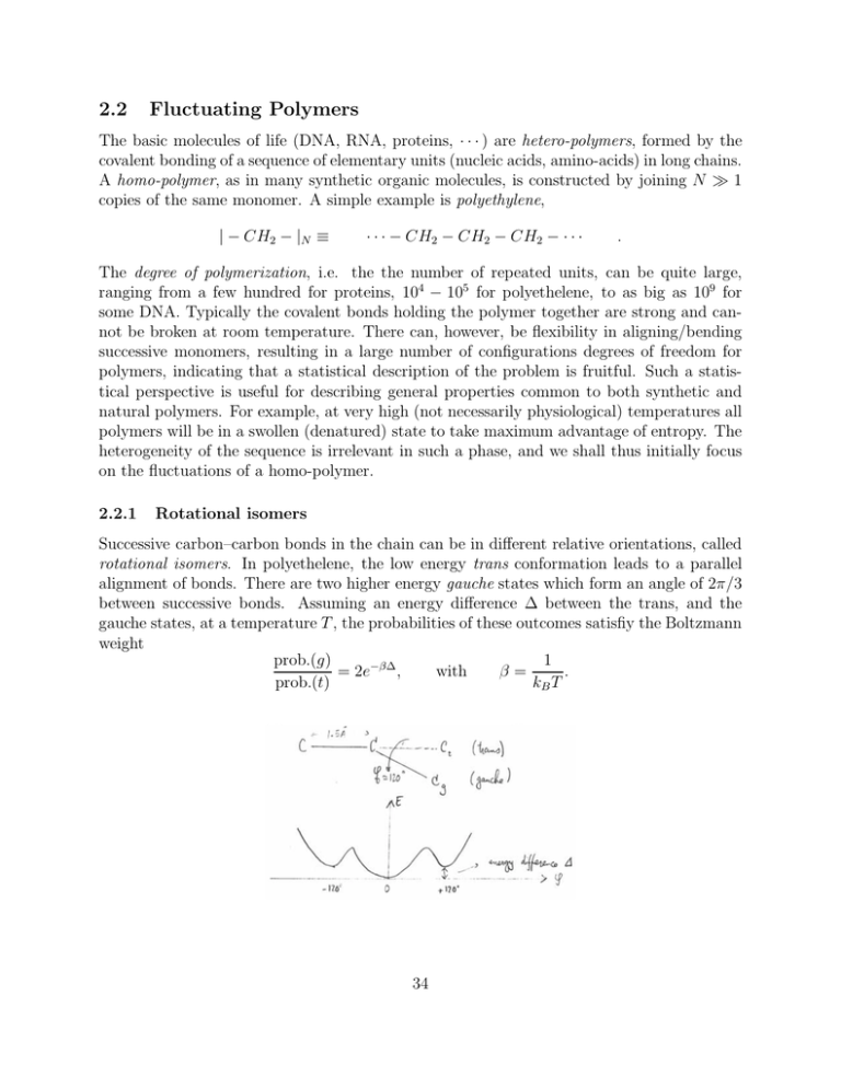
Successive carbon–carbon bonds in the chain can be in different relative orientations, called
rotational isomers. In polyethelene, the low energy trans conformation leads to a parallel
alignment of bonds. There are two higher energy gauche states which form an angle of 2π/3
between successive bonds. Assuming an energy difference ∆ between the trans, and the
gauche states, at a temperature T , the probabilities of these outcomes satisfiy the Boltzmann
weight
prob.(g)
1
= 2e−β∆ ,
with
β=
.
prob.(t)
kB T
34
For (CH2 )N , ∆ is quite small (roughly 500 cal/mole or 1/3kB T ), and the polymer is
very flexible at room temperature. For other polymers ∆ > kB T , and gauche states with
probability
e−β∆
p(g+ ) = p(g− ) =
,
1 + 2e−β∆
are relatively rare. A typical configuration then consists of long straight segments with few
bends. The probability of a straight segment of n monomers is pnt (1−pt ), where pt = 1−2p( g)
is the probability of a trans bond. The average length of straight segments is thus hnia, where
a is the bond length (monomer size), and
hni = −
−1
1
= ln 1 + 2e−β∆
.
ln pt
(2.28)
The typical size of these linear segments is proportional to the persistence of the polymer.
The persistence length characterizes the decay of orientational correlations along the chain.
In the above simplified model, let us denote the orientation of the bonds by the set of vectors
{~t1 , ~t2 , · · · , ~tN }, with ~tj · ~tj = a2 . Assuming that the (two) gauche states produce a relative
bond angle φ, we have
−β∆
2
−β∆
~t1 · ~t2 = a2 1 + 2 cos φe
≈
a
exp
−2(1
−
cos
φ)e
,
1 + 2e−β∆
where the last expression is valid in the limit of β∆ ≫ 1 where a gauche state is very unlikely.
In the same approximation, the correlation between bonds that are further apart is given by
−β∆
+ O(e−2β∆ )
2
−β∆
~t1 · ~tn+1 ≈ a2 1 + 2n cos φe
≈
a
exp
−2n(1
−
cos
φ)e
,
1 + 2ne−β∆ + O(e−2β∆ )
where we have included only configurations with one gauche bond. The orientation correlations decay exponentially as e−ℓ/ξp , where ℓ = na is the counter-length along the polymer,
and the persistence length ξp is given by
ξp ≈
2.2.2
aeβ∆
.
2(1 − cos φ)
(2.29)
Worm-like chain
For a rigid polymer such as double-stranded DNA a kink causing a finite rotational angle is
energetically costly and does not occur. The loss of angular correlations at long distances
then occurs from the accumulation of small changes from one monomer to the next. If
we indicate as before a polymer configuration by the set of vectors {~t1 , ~t2 , · · · , ~tN }, we can
approximate the energy of a nearly straight configuration by
H = −J
N
−1
X
i=1
35
~ti · ~ti+1 , .
(2.30)
Since in a typical configuration ~t changes slowly, it is useful to go over to a continuum limit in
which the discrete monomer index i is replaced by the continuous arc-length s ∈ [0, L = Na].
2
Using ~ti − ~ti+1 = 2 − 2~ti · ~ti+1 , we then can write
κ
H ≈ −JN +
2
Z
L
0
d~t
ds
ds
2
,
(2.31)
where κ = J/a is the coefficient of bending rigidity. (Note that |d~t/ds| = 1/R(s), where R(s)
is the local radius of curvature.)
Ignoring the initial energy of the “ground state” configuration, it is common to write the
energy in dimensionless form as
ξp
βH = −
2
Z
L
0
ds
d~t
ds
2
,
(2.32)
with βκ = ξp . We have anticipated that the bending rigidity is related to the persistence
length. In fact, it can be shown (e.g. by using transfer matrices) that for the discrete model
of Eq. (2.30)
|m−n|
1
~
~
(2.33)
htm · tn i ≈ coth(βJ) −
for |m − n| ≫ 1,
βJ
and thus in the continuum limit
h~t(s) · ~t(s + ℓ)i ≈ e−ℓ/ξp ,
(2.34)
with ξp ≈ βκ for βJ ≫ 1. This, so called worm-like chain model is frequently invoked as a
description of double-stranded DNA, where ξp is in the range of 50-100nm.
2.2.3
Entropic elasticity
The flexibility of long polymers arises from the statistical fluctuations of segments larger than
the persistence length. The important parameter that governs the number of configurations
is thus not the degree of polymerization N, but the number of unconstrained degrees of
freedom, or the Kuhn length NK ≈ Na/(2ξp ). To see this explicitly, let us consider the end
to end separation of the polymer, given by
~ = ~t1 + ~t2 + · · · + ~tN =
R
36
N
X
i=1
~ti .
~ = 0,
Because of rotational symmetry (there is no cost for rotating the entire polymer), hRi
and its variance is given by
hR2 i =
N
X
h~ti · ~tj i = Na2 + 2
i,j=1
X
i<j
h~ti · ~tj i .
(2.35)
We shall assume that the orientational correlations decay as a simple exponential (this is
only asymptotically correct), i.e.
h~ti · ~tj i = a2 e−a|i−j|/ξp .
(2.36)
As the correlation function is the same for every pair of points separated by a distance k,
and as there are (N − k) such pairs along the chain
2
2
2
hR i = Na + 2a
N
X
k=1
(N − k)e−ak/ξp .
(2.37)
The geometric series are easily performed, and for N ≫ 1 (where only the term proportional
to N is significant), we obtain
2e−a/ξp
a
2
2
2
hR i = Na 1 +
= Na coth
(2.38)
1 − e−a/ξp
2ξp
Na
2
≈ 2Naξp = (2ξp )
.
(2.39)
2ξp
The approximations in the second line rely on ξp ≫ a. The very last expression indicates
that the behavior of the variance is the same as that of NK ≡ (Na/2ξp ) independent rods
of length 2ξp , i.e. the same variance is obtained for a collection of NK freely–jointed rods,
each of length 2ξp . Indeed the correlations between these Kuhn segments is sufficiently small
that in the limit of NK ≫ 1, we expect the Central Limit Theorem to hold, leading to the
probability distribution function
3/2
2
2
2
3R
2πhR
i
3R
1
~ = exp −
p(R)
= exp −
.
2
2hR i
3
4Naξp (4πNaξp /3)3/2
(2.40)
The final probability distribution is identical to the Boltzmann weight of a Hookian spring of
strength J connecting the end points of the polymer, and the result of entropic fluctuations
can be interpreted as conferring an elastic bond between the ends of the polymer with spring
coefficient
3kB T
3kB T
Jpolymer =
=
.
(2.41)
2
hR i
2Naξp
37
2.3
Interacting Polymers
The polymeric properties discussed so far arose from the flexibility of the covalent bonds
that join adjacent monomers. There are also interactions between any other pairs (triplets,
etc.) of monomers which depend on their spatial vicinity and that favor certain spatial
configurations. Indeed, it is such interactions, typically due to hydrogen bonds, that enable
proteins to fold and assume specific shapes. There are competing effects due to thermal
fluctuations and competition with solvent interactions.
Some of the ingredients of polymer interactions in a solvent is present in the very simple
model of chain configurations on a (say square) lattice. The set of random walks on the
square lattice that do not step back to the previous site grows with the number of steps N
as 3N . One simple consequence of interactions is that it is physically impossible to visit a
previously occupied site. The constraint of excluded volume prunes the random walks to a
smaller subset of so-called self-avoiding walks. The number of self-avoiding walks also grows
exponentially as g N with g < 3 (g ≈ 2.64).
A simple way to incorporate interactions on a lattice is to count the number of (nonpolymeric) nearest-neighbor pairs, and assign energy
E = ǫmm Nmm + ǫms Nms + ǫss Nss ,
where mm, ms, and ss stand for monomer-monomer, monomer-solvent, and solvent-solvent
pairs respectively, with Npair and ǫpair indicating the corresponding number and bondenergies. As two initially separate monomers are brought into contact, two ms bonds
are replaced by one mm bond and one ss bond, leading to a change in energy of δǫ =
ǫmm + ǫss − 2ǫms . The preference of the monomers to aggregate in solvent is thus captured
by the dimensionless “Flory–Huggins” parameter
β
ǫmm + ǫss
.
(2.42)
χ ≡ − δǫ = β ǫms −
2
2
A negative χ leads to separation of monomers, while a positive χ encourages their aggregation.
38
In a more realistic model, the interactions between molecules vary continuously as a
function of their relative separation and orientation in space. The dependence on orientation
is particularly relevant to hydrogen bonding, while the van der Waals attraction mainly
depends on the separation. Just as in Eq. (2.8), an effective potential V(r) between monomers
is in principle obtained by integrating over all positions (and orientations) of the solvent
particles. In the usual case where the monomers are larger than the solvent molecules, the
effective potential is attractive at large distances and has a hard repulsive core at short
distances. For a good solvent the potential is weak, while a strong attractive potential favors
aggregation of monomers in a bad solvent. The quality of solvent also changes as a function
of temprature due to entropic contributions of its constituents. The larger entropy of solvent
molecules typically improves the quality of a solvent at higher temperatures.
2.3.1
Mean-field estimate of the partition function
To calculate the properties of a polymer in solvent– e.g. to determine if it is in its native
form or a denatured state at some temperature– we need to compute the free energy of the
molecule and it environment. Computation of the partition function is a hard task, even
for the highly simplified models we have introduced so far. We shall instead rely upon an
approximate expression obtained in a mean-field/variational treatment. Let us assume that
the most likely configurations of an interacting homopolymer have a typical size R. The
partition of N monomers confined to a sphere of radius R is then estimated as
3R2
exp − 4N
aξp
Z(N, R) ≈ g N ×
(2.43)
(4πNaξp /3)3/2
a 3 a 3 a 3 ×
1· 1−
· 1−2
· · · 1 − (N − 1)
× e−βEatt. .
R
R
R
The first line in Eq. (2.44) pertains to the entropy of the polymer, the first term encodes
the exponential growth in the number of configurations of an unconstrained polymer– the
39
precise value of g is in fact irrelevant to the considerations that follow. The second term
approximates the reduction in the number of configurations when the polymer is constrained
to a size R. The effect of this reduction is included as a Hookian spring, motivated by the
result in Eq. (2.40) for the end-to-end probability of a non-interacting polymer.
The second line in Eq. (2.44) approximates the effect of interactions and is broken into two
parts. The first part encodes the reduction in phase space due to excluded volume constraints:
the first monomer is unconstrained, the volume available to the second is reduced by the
fraction (a/R)3 due to the volume excluded by the first, and so on. The reductions due to
the excluded volume make a contribution to the free energy proportional to
δ ln ZEV =
N
−1
X
i=1
a 3 X
a 3 1 a 6 X 2
ln 1 − i
≈ −
i−
i +···
R
R
2 R
N 2 a 3 N 3 a 6
−
−··· .
≈ −
2 R
6 R
The attractive part of the interaction, for homopolymers, is given by
Z
1X
1
V(~ri − ~rj ) =
d3~rd3~r′ n(~r)n(~r′ )V(~r − ~r′ ) .
Eatt. =
2
2
(2.44)
(2.45)
i6=j
Assuming a uniform mean-density, n(~r) = n = N/V = N/(4πR3 /3), leads to
Z
n2
Eatt. = V
d3~rV(~r) ,
2
a
(2.46)
where we have integrated over the center of mass of the pair to get the volume V , and
ignored any contributions from the surface. In the spirit of Flory-Huggins, we introduce a
dimensionless parameter χ, via
Z
4π 3
3
d ~rV(~r) ≡ − a kB T (2χ) ,
(2.47)
3
a
to capture of the net effect of attractions, and such that
a 3
−βEatt. = N 2
χ.
R
The resulting free energy, with R as a variational parameter,
3
4πNaξp
3R2
ln Z(N, R) = N ln g − ln
−
2
3
4Naξp
a 3
2 3
3 6
N
a
N
a
−
−
− · · · + χN 2
.
2 R
6 R
R
will next be used to explore the phases of the interacting homopolymer.
40
(2.48)
(2.49)
0,72SHQ&RXUVH:DUH
KWWSRFZPLWHGX
-+67-6WDWLVWLFDO3K\VLFVLQ%LRORJ\
6SULQJ
)RULQIRUPDWLRQDERXWFLWLQJWKHVHPDWHULDOVRURXU7HUPVRI8VHYLVLWKWWSRFZPLWHGXWHUPV