1.204 Lecture 19
Continuous constrained nonlinear
optimization:
optimization:
Convex combinations 2:
Network equilibrium
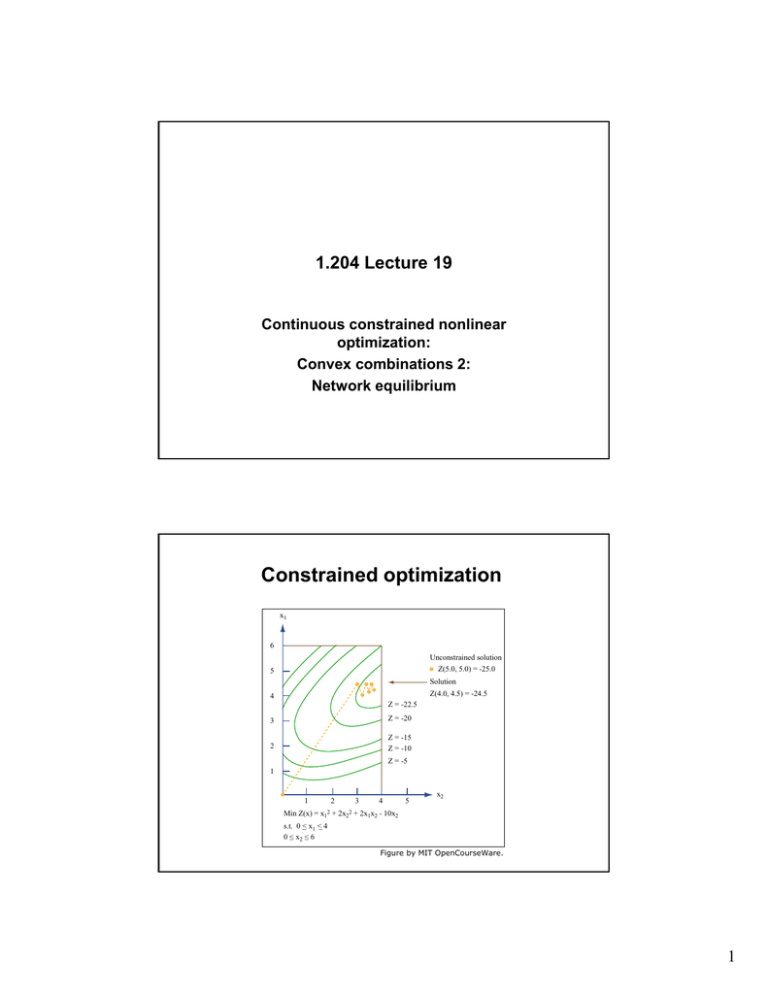
Constrained optimization
x1
6
Unconstrained solution
Z(5.0, 5.0) = -25.0
5
Solution
Z(4.0, 4.5) = -24.5
4
Z = -22.5
3
Z = -20
2
Z = -15
Z = -10
Z = -5
1
1
2
3
4
5
x2
Min Z(x) = x12 + 2x22 + 2x1x2 - 10x2
_ x1 <_ 4
s.t. 0 <
_ x2 <
_6
0<
Figure by MIT OpenCourseWare.
1
Network equilibrium problem formulation
min z(x) =
∑
xa
t
∫ ta (ω ) dω
arcs a 0
∑f
rs
k
= qrs
Link Travel Time [min]
subject to
∀OD pairs r, s
paths k
Free flow travel time
f krs ≥ 0 ∀k, r, s
xa = ∑
i
∑ ∑f
j
∀r,, s,, k
rs
k
X3
Capacity
ω
Link Flow [veh/hr]
k
Figure by MIT OpenCourseWare.
if a on path from r to s
Figures, examples from Sheffi
Convex combinations algorithm 1
• Applying the convex combinations algorithm
requires solution of a linear program at each step
min z n ( y) =
∂z(x n )
⋅ ya
arcs a ∂xa
∑
for all feasible y
• Gradient of z(x) is just the arc travel times:
∂z(x n ) n
= ta
∂xa
• The linear program becomes:
min z n ( y) = ∑ t an ⋅ ya
s.t.
∑g
a
rs
k
= qrs
∀r, s
k
g krs ≥ 0 ∀k, r, s
ya = ∑
rs
∑g
rs
k
∀a in path
k
t an = t a (xan )
2
Convex combinations algorithm 2
• The linear program minimizes travel times over a
network with fixed, not flow-dependent times.
– Total time is minimized by assigning each traveler to
shortest O-D path
– Thus, a shortest path algorithm, plus loading flow on the
links used by each O-D pair, solves the linear program
• Line search step uses bisection method which,
for a minimization problem, requires a derivative
– It happens to be easy to compute. After a lot of algebra:
∂
z[x n + α ( y n − x n )] = ∑ ( yan −xan ) t a (xan + α ( yan − xan ))
∂α
a
Convex combinations steps
• Step 0: Initialization.
– Find shortest paths based on ta=ta(0).
– Assign flows to obtain {xa1}
• Step 1:
1 Update times.
times
– Set tan=ta(xan) for all a
• Step 2: Direction finding.
– Find shortest paths based on {tan}
– Assign flows to obtain auxiliary flows {yan}
• Step 3: Line search. Find αn that solves
–
min ∑
0≤α ≤1
a
xan +α ( y an − xan )
∫t
a
(ω )dω
0
• Step 4: Move. Set
x n+1 = x n + α n ( y n − x n )
• Step 5: Convergence test. If not converged, go to step 1
3
Example network
Link 1
O
D
Link 2
Link 3
x
t1 = 10 [ 1 + 0.15 ( 1 )4 ] Time units
2
x2 4
t2 = 20 [ 1 + 0.15 ( ) ] Time units
4
x3 4
t3 = 25 [ 1 + 0.15 ( ) ] Time units
3
x1 + x2 + x3 = 10 Flow units
Figure by MIT OpenCourseWare.
Example program output
Iter
Step
0 Update
Move
1
2
3
4
5
t:
x:
Link:
1
10.0
10.00
2
20.0
0.00
Update
Direction
Move
t:
y:
x:
947.5
947
5 20.0
20 0
0.00 10.00
4.03 5.97
Update
Direction
Move
t:
y:
x:
34.8
0.00
3.38
Update
Direction
Move
t:
y:
x:
22.3
10.00
3.62
Update
Direction
Move
t:
y:
x:
26.1
0.00
3.55
Update
Direction
Move
t:
y:
x:
24.8
10.00
3.59
3
Objective fn
25.0
0.00
0.00
25.0
25 0
0.00
0.00
1975.00
1975 00
34.8 25.0
0.00 10.00
5.00 1.61
197.40
27.3
0.00
4.83
25.3
0.00
1.55
189.99
26.4 25.3
0.00 10.00
4.73 1.73
189.45
25.9
0.00
4.69
189.36
25.4
0.00
1.71
Alpha
0.597
0.161
0.036
0.020
0.007
4
NetworkEquilibrium data members
public class NetworkEquilibrium implements MathFunction {
public static final int EMPTY= Short.MIN_VALUE;
private int nodes;
p
;
private int arcs;
private int[] head;
// Graph data structure
private int[] to;
// Graph data structure
private double[] timeBase;
// Zero flow time
private double[] timeExponent;
// 4 in our example
private double[] timeConst;
// .015/lanes in example
private double[] D;
// Distance from root
private int[] P;
// Predecessor node back to root
private
i t int[]
i t[] Parc;
P
// P
Pred
decessor arc back
b k to root
t
private double[] xFlow; // Arc flows
private double[] yFlow; // Auxiliary arc flows
private double[] arcTime;
// ta
private double[][] ODtrips;
// qrs
// This Java code is tested only on our simple example
// It should be basically correct for larger problems, but…
NetworkEquilibrium constructor
NetworkEquilibrium(int n, int a, int[] h, int[] t,
double[] tBase, double[] tExponent, double[] tConst,
double[][]
[][] od)
) {
{
nodes= n;
arcs= a;
head= h;
to= t;
timeBase= tBase;
timeExponent= tExponent;
timeConst= tConst;
ODtrips= od;
arcTime=
Ti
new double[arcs];
d bl [
]
}
5
Changes in shortest path
• Time is method, not data from array.
– Replace dist in original version with time()
• Times are double, not int variables
– Ints are faster, but doubles are easier
• Must keep track of predecessor arc as well as
predecessor node in shortest path tree result
– There may be multiple arcs
• Method is private
Shortest path
private void shortHKNetwork(int root) {
// root is argument
final int MAX_COST= Integer.MAX_VALUE/2;
final int NEVER_ON_CL= -1;
final int ON_CL_BEFORE
ON CL BEFORE= -2;
2; final int END_OF_CL= Integer.MAX_VALUE;
D= new double[nodes];
// double, not int
P= new int[nodes];
Parc= new int[nodes];
// May be >1 arc between nodes
int[] CL= new int[nodes];
for (int i=0; i < nodes; i++) {
D[i]= MAX_COST; P[i]= EMPTY;
Parc[i]=
[i] EMPTY;
CL[i]= NEVER_ON_CL; } // Initialize root node
D[root]= 0;
CL[root]= END_OF_CL;
int lastOnList= root;
int firstNode= root;
6
Shortest path 2
do {
double Dfirst= D[firstNode];
for (int link= head[firstNode]; link < head[firstNode+1]; link++) {
int outNode= to[link];
double DoutNode= Dfirst+ time(link); // Compute time()
if (DoutNode < D[outNode]) {
P[outNode]= firstNode;
Parc[outNode]= link;
// Record new predecessor arc
D[outNode] DoutNode;
D[outNode]=
int CLoutNode= CL[outNode];
if (CLoutNode == NEVER_ON_CL || CLoutNode == ON_CL_BEFORE) {
int CLfirstNode= CL[firstNode];
if (CLfirstNode != END_OF_CL && (CLoutNode == ON_CL_BEFORE ||
DoutNode < D[CLfirstNode])){
CL[outNode]= CLfirstNode;
CL[firstNode]= outNode; }
else {
CL[
[lastOnList]
]= outNode;
;
lastOnList= outNode;
CL[outNode]= END_OF_CL; }
}
}
}
int nextCL= CL[firstNode];
CL[firstNode]= ON_CL_BEFORE;
firstNode= nextCL;
} while (firstNode < END_OF_CL); }
equilibrium()
public void equilibrium() {
final double CRITERION= 0.001;
// Convergence criterion
final int MAX_ITERATIONS= 10;
// Set higher in real code
// Step 0: Initialization
xFlow= new double[arcs];
// Initialize xFlow = 0
update();
xFlow= directionFind();
double convergence;
int iterations= 0;
do {
// Step 1: Set times based on initial flows
update();
// Step 2: Direction finding
yFlow directionFind();
yFlow=
directionFind();
// Step 3: Line search
double alpha= lineSearch(this, 0.0, 1.0); // 0 <= alpha <= 1
// Step 4: Move
convergence= move(alpha);
// Step 5: Check convergence
iterations++;
} while (convergence > CRITERION && iterations < MAX_ITERATIONS);
}
7
update(), time()
private void update() {
for (int i= 0; i < arcs; i++) {
arcTime[i]=
[ ] time(i);
( );
}
}
private double time(int link) {
final double TOLERANCE= 1E-8; // Sqrt of machine precision
double time;
if (xFlow[link] < TOLERANCE)
time= timeBase[link];
el
lse {
double delay= 1.0 + timeConst[link]*
Math.pow(xFlow[link], timeExponent[link]);
time= timeBase[link]*delay;
}
return time;
}
directionFind()
private double[] directionFind() {
double[] flow= new double[arcs];
// Assign trips on shortest path (set of arcs)
for (int i
i= 0; i < nodes; i++) { // Loop thru origin nodes
shortHKNetwork(i); // Shortest path from i to all nodes
for (int j= 0; j < nodes; j++) {
if (i != j) {
int pred= P[j];
while (pred != EMPTY) {
// While not back at root
// Add this flow to arcs in shortest path from O to D
flow[Parc[j]] += ODtrips[i][j];
// Find previous arc on path, until we reach the root
pred=
d P[pred];
[
d] }
}
}
}
return flow;
// We have flows on all arcs, based on current travel times
}
8
lineSearch()
// Uses d.derivative—see next slide
private double lineSearch(MathFunction d, double a, double b) {
final double TOLERANCE= 1E-8;
1E 8; // Square root of machine precision
final double MAX_ITERATIONS= 1000;
double m;
// Midpoint
int counter= 0;
for (m= (a+b)/2.0; Math.abs(a-b) > TOLERANCE; m= (a+b)/2.0) {
counter++;
if (d.derivative(m)< 0.0)
// If derivative negative,
a= m;
// Use right subinterval
else
b m;
b=
// Use left
l f subinterval
bi
l
if (counter > MAX_ITERATIONS)
break;
}
return m;
}
// There are better line searches such as Brent’s method (see
// Numerical Recipes 10.2-10.4) but bisection is simple and stable
derivative()
public double derivative(double alpha) {
final double TOLERANCE= 1E-8;
double deriv= 0.0;
for (int i= 0; i < arcs; i++) {
double time;
double newFlow= xFlow[i]+ alpha*(yFlow[i]- xFlow[i]);
if (newFlow < TOLERANCE)
time= timeBase[i];
else {
double delay= 1.0 + timeConst[i]*
Math.pow( newFlow, timeExponent[i]);
time= timeBase[i]*delay;
}
deriv += (yFlow[i] - xFlow[i])*time;
}
return deriv;
}
public interface MathFunction {
double derivative(double alpha);
}
9
move(), main()
private double move(double alpha) {
double sumFlows= 0.0;
double sumRootMeanDiffFlows= 0.0;
;
for (int i= 0; i < arcs; i++) {
double flowChange= alpha*(yFlow[i] - xFlow[i]);
xFlow[i]+= flowChange;
sumFlows+= xFlow[i];
sumRootMeanDiffFlows+= flowChange*flowChange;
}
// Compute convergence criterion here, since we have
// current and previous xFlow
return
t
Math.sqrt(sumRootMeanDiffFlows)/sumFlows;
M th
t(
R tM
DiffFl
)/
Fl
}
public static void main(String[] args) {
NetworkEquilibrium g= new NetworkEquilibrium();
g.equilibrium();
}
Summary
• Convex combinations method (also known as Frank-Wolfe
decomposition) solves network equilibrium problem
– Flow taken from more congested paths
paths, assigned to less
congested paths, until flow changes are small
– Process equalizes travel times on all paths for O-D pair
– Uses shortest path code to solve linear program subproblem
• Shortest path is very efficient even for large networks
– Convex combinations method converges slowly
• Faster methods exist but require more data storage and don’t use
shortest path subproblem as naturally
• Note the building blocks:
– Shortest path algorithm, which uses graph, queue (candidate
list) and tree data structures
– Line search is a bisection (divide and conquer) algorithm
– NetworkEquilibrium is the master problem, solved by reusing
the building blocks listed above
– Having a library of data structures and core algorithms is key
to problem solving and design
10
Performance of convex combinations
Y
Start
X
Successive minimizations along coordinate directions in a long, narrow valley
Figure by MIT OpenCourseWare.
Numerical Recipes
Performance of convex combinations
• Convergence is slow, even in our 3 link example
– Objective function value changes little
little, but flows and
times are accurate to only 2 places after 9 iterations
• Complexity is measured in two dimensions
– Typical performance ~O(n), where n is number of arcs:
• Running time increases linearly in usual experience
– Linear convergence is claimed:
• εn+1= k εnm , m = 1
• It depends on definition of ε
– Objective function converges linearly
– Arc flows and times appear to converge sublinearly
• Linear convergence means each iteration gains one more
significant figure
– Sublinear means less than one more significant figure
– Superlinear means more than one more significant figure
11
Congestion
• Highway networks have diseconomies of scale in urban
areas
– Congestion is major element in urban form
form, environmental
quality, urban economics (agglomeration), and travel behavior
– More trips mean lower service quality
• Transit networks on separate rights of way are often
regarded as having economies of scale
– More trips mean higher service frequency, which gives higher
service quality
– Eventually congestion occurs in transit also, as capacity is
approached
• Extensions of network equilibrium formulations handle
highway-transit demand equilibrium, variable demand, …
– Sheffi covers many of them
– Regional trade, etc. can also be modeled this way
12
MIT OpenCourseWare
http://ocw.mit.edu
1.204 Computer Algorithms in Systems Engineering
Spring 2010
For information about citing these materials or our Terms of Use, visit: http://ocw.mit.edu/terms.