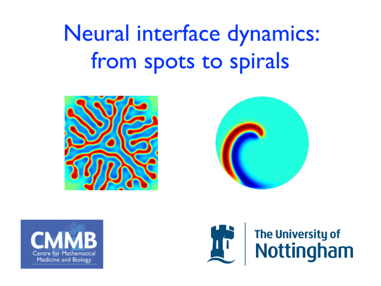
Neural interface dynamics: from spots to spirals
Brain and Cortex
Principal cells and interneurons
Santiago Ramón y Cajal
1900
Eugene Izhikevich 2008
Electroencephalogram (EEG) power spectrum
EEG records the activity of ~ 106 pyramidal neurons. Population model
Firing rate activity f(E)
WEE
PE
E
WEI
PI
WIE
h
I
WII
Ė =
Firing rate activity f(I)
E
+
E
İ =
I
I
+ WEE gEE (A
+ WII gII (A
E) + WEI gEI (A
I) + WIE gIE (A+
E) + PE
I) + PI
WEE
PE
WEI
⇥(t) =
2
te
Q⇥ =
E
Q=
PI
WIE
I
QgjE = f(E)
Steady state
approximation
Qg = f
f = f ({g})
⇥2
t
0
WII
1 d
1+
dt
t
QgjI = f(I)
E = E(gEE , gEI )
g=
I = I(gII , gIE )
f
Alphoid chaos (10 D)
p
o
w
e
r
frequency
PI
LLE (S
1
)
inhibition
Shilnikov saddle-node route to chaos
excitation
van Veen and Liley, PRL, 97, 208101 (2006)
P
Spatially extended models
g=w⇥
f
Simplest neural field model: Wilson-Cowan (‘72), Amari (‘77)
f(u(x, t ⇤ |x ⇤ y|/v))
g = u(x, t)
x
u(x, t) =
w(|x ⇤ y|)
dy w(y)
y
ds (s) f (u(x ⇤ y, t ⇤ s ⇤ |y|/v))
0
uab =
⇥ab
ab
2D layers
b
ha =
uab
b
wab
a
p
o
w
e
r
frequency
ab (r, t)
=
R2
dr wab (r, r )fb hb (r , t ⇤ |r ⇤ r |/vab )
Turing instability analysis
E layer and I layer
e
ik·r
e
t
Continuous spectrum
det (D(k, ) ⇤ I) = 0
[D(k, ⇤)]ab = ⇥ab (⇤)Gab (k, ⇤i⇤)
= LT
G = FLT w(r) (t ⇤ r/v)
S Coombes et al., PRE, 76, 05190 (2007)
b
= f (ss)
Re (k)
0.2
= ⇥ + i⇤
0
2
4
i
(k)
6
8
0
6
i
4
6
2
4
0
2
0
a.
20
0
0.2
0
2
15
Turing-Hopf
4
6
10
8
6
c
Hopf
5
4
6
2
4
0
0
2
0
b.
0
2
4
6
8
v (axonal speed)
10
12
c
Amplitude Equations (one D)
Coupled mean-field Ginzburg–Landau equations describing a
Turing–Hopf bifurcation with modulation group velocity of O(1).
2
⇤A1
⇤ A1
2
2
= A1 (a + b|A1 | + c |A2 | ⇥) + d 2
⇤⇥
⇤ +
2
⇤A2
⇤
A2
2
2
= A2 (a + b|A2 | + c |A1 | ⇥) + d 2
⇤⇥
⇤
Benjamin–Feir (BF)
t
BF-Eckhaus instability
t
x
k
k
Coefficients in terms of integral transforms of w and
.
Applications to co-registered EEG/fMRI
Ingo Bojak
Bojak, I., Oostendorp, T. F., Reid, A. T., Kotter, R., 2009. Realistic mean field forward predictions for the
integration of co-registered EEG/fMRI. BMC Neuroscience 10, L2.
A simple 2D neural field model
R
ut (x, t) =
2
u(x, t) +
R2
w(x
x )H[u(x , t)
2D Amari model
Neural Fields: Theory and Application, (531 pages)
Ed. S Coombes, P beim Graben, R Potthast and J J Wright, Springer Verlag, June 2014
h]dx
A simulation
An interface is easily identified
Interface dynamics in 2D
n(s)
B
s
r(s)
n=
n(s )
x u|
r(s )
ut (x, t) =
t(s )
t(s)
x u/|
s
B
u(x, t) + (x, t)
(x, t) =
w(|x
x |)dx
B(t)
Differentiate u(x, t) = h along B(t)
Normal velocity
dr
u
+
=0
xu ·
dt
t
dr
ut
n·
=
dt
|z|
z
⇥x u(x, t)|x=r
ut =
dx w(|r
h+
⇥
x |),
B
zt =
z+
dx w(|x
x
x |)
B
x=r
n
=
B
B
K0 - Bessel function of the second kind
2
(1
)K0 (x) = 2⇥ (x)
N
w(r) =
⇥
⇥
i r)
i=1
dx
x w(|x
x |) =
B
dx K0 ( |x
B
Ai K 0 (
dsn(s)w(|x
x (s)|)
B
x |) =
1
x
dsn(s) ·
|x
B
r(s)
K1 ( |x
r(s)|
r(s)|) + C
2⇥
2
Dynamics from data on the boundary only
For points on the boundary parametrised by s
⇥
⇤
N
⌅
⇥
ut (s) = h +
Ai
ds n(s ) · Ri (s, s ) + 2
B
i=1
zt (s) =
⇤
z(s)
Ri (s, s ) =
n(s)
B
s
r(s)
ds n(s )w(|r(s)
r(s )|)
B
1 r(s)
i |r(s)
r(s )
K1 (
r(s )|
i |r(s)
r(s )|)
n(s )
r(s )
t(s )
t(s)
i
s
Biot-Savart style interaction
B
[effective repulsion between two arc length
positions with anti-parallel tangent vectors]
Simple numerical scheme
Stability of stationary states
B0
Zero normal velocity - ut = 0, B(t)
⇥
⇧
⇤
N
⌅
⇥
h=
dx w(|r x |) =
Ai
ds n(s ) · Ri (s, s ) + 2
B0
i=1
B0
i
ut = 0
B0
B0
u(t) = u|x
B
u|x
B0
u(B0 ) = h
B
defines R = R + R(⇥, t)
B
u(B) = h
=0
Spots
2R
h = 2⇥
N
⇤
Ai
i=1
10
Using Graf’s formula:
1
2
i
R
⇥m =
m=4
m=3
6
m=3
γ=5
γ=4
4
m=2
m=2
m=2
γ=3
2
0
0
0.05
0.1
K1 (
i R)I0 ( i R)
i
R(⇥, t) = cos m⇥e
m=4
8
R
0.15
h
0.2
1+
⇥
mt
N
i=1 Ai Km ( i R)Im ( i R)
N
i=1 Ai K1 ( i R)I1 ( i R)
Stripes (Mex-hat)
u(x, y1 ) = h = u(x, y2 )
yi = yi +
i cos(kx)e
t
λ
0.1
0
sinuous
-0.1
varicose
-0.2
0
0.2
0.4
0.6
0.8
k 1
Linear adaptation
1
ut =
u+⇥
at = u
ga,
a
Exploit linearity
t
t
ds (t
u(·, t) =
⇥(t) =
⇤
⇥± =
⇤+
1+
dse
s)⇥(·, s), a(·, t) =
+t
(1
⇤+ )e
±
(1 + )2
2
Easy to construct stationary spots
(1
(t s)
⇤ )e
u(·, s)
⇥
t
4 (1 + g)
h
h(1 + g)
Instabilities and travelling pulses
Eigenvalues determined by Em ( ) = 0
1
Em (⇥) =
(⇥)
Wm
(1 + g)Wm
R
=
|⇥ (R)|
e
(⇥) =
s
(s)ds
0
2
d cos(m )w(R( ))
0
m = 0 mode ( = i⇥ , breath) unstable when g > 1/
emergent frequency ⇥ =
m=1
mode (
g
1
R , drift) unstable when g > 1/
Breathing
a
b
c
3
b
2.5
2
0
e
a
R(t)
e
d
d
c
5
10
15
20
25
30
t
35
40
Drifting
… at the point where g = 1/ the shape of the spot deviates from
circular with an amplitude that depends on quadratic and higher powers of c
m
R( ) = R +
c am cos m
m 2
Lu Y, Amari S: Traveling bumps and their collisions in a 2D neural field. Neural Computation 2011, 23:1248–1260
Drifting (weakly nonlinear analysis)
For any sigmoid drifting will occur when g increases
through 1/
Amplitude analysis
(translation operator and drift eigen-modes):
2
X(r, t) = (p) 4S(r) +
2
X
j=1
p denotes location of spot
ṗ = a
3
aj (t)⇤j (r) + ⇥(r, t)5
a = a1 + ia2
2
ȧ = a(M1 |a| + M2 )
00
1 000 3
†
⇥M1 = F ⌅1 | ⇤1 ⇥ + F ⌅1 V12 | ⇤†1 ⇥ + ⇧x1 V1 | ⇤†1 ⇥,
6
00
⇥M2 = F ⌅1 V4 | ⇤†1 ⇥ +
(S)⌅1 | ⇤†1 ⇥ + ⇧x1 V4 | ⇤†1 ⇥
spare the details!
Scattering
Two spots with centers offset by a vector h = 2p
3
ṗ = a + G0 f(p),
ȧ = M1 a + M2 a + H0 f(p),
f(p) = e
z = f(p)
-2p
0.1
z
t= 0
0.05
3.75
7.5
11.25
/
p
15
2p
18.75
22.5
0.3
0
u
-0.05
a = velocity
-0.1
-0.3
-0.15
0
0.15 a 0.3
−0.1
Spirals
Spiral Waves in Disinhibited Mammalian Neocortex (rat slice)
Huang et al., J Neurosci. 2004
An interface approach (in progress)
Look for rigidly rotating solutions of the form
Shape of the spiral arm determined by
Stability:
… watch this space!
In collaboration with
Helmut Schmidt
Ingo Bojak
(Exeter)
(Reading)
Daniele Avitabile and Aytül Gökçe
(Nottingham)
The Journal of Mathematical Neuroscience
The Journal of
Mathematical
Neuroscience
S Coombes, H Schmidt and I Bojak 2012
Interface dynamics in planar neural field
models.
EDITORSINCHIEF
Stephen Coombes
Olivier Faugeras
COMING
IN
2011
EDITORIAL BOARD
Shun-ichi Amari
Peter Ashwin
Paul Bressloff
Romain Brette
Bard Ermentrout
Wulfram Gerstner
Vincent Hakim
David Holcman
Viktor Jirsa
Carlo Laing
André Longtin
Hinke Osinga
Andrey Shilnikov
David Terman
John Terry
Martin Wechselberger
AIMS AND SCOPE
The Journal of Mathematical Neuroscience (JMN) publishes research articles on the
mathematical modeling and analysis of all areas of neuroscience, i.e., the study of
the nervous system and its dysfunctions.
The focus is on using mathematics as the primary tool for elucidating the fundamental mechanisms responsible for experimentally observed behaviours in neuroscience at all relevant scales, from the molecular world to that of cognition. The aim
is to publish work that uses advanced mathematical techniques to illuminate these
questions.
It publishes full length original papers, rapid communications and review articles.
Papers that combine theoretical results supported by convincing numerical experiments are especially encouraged. Papers that introduce and help develop those new
pieces of mathematical theory which are likely to be relevant to future studies of the
nervous system in general and the human brain in particular are also welcome.
Now accepting submissions: www.springer.com/13408