Approximately optimal importance sampling for Λ–coalescents
Jere Koskela, Paul Jenkins and Dario Spanò
Mathematics Institute and Department of Statistics, University of Warwick
Introduction
Ancestry as missing data
The Λ–coalescent family ([Pit99], [Sag99]) models the ancestry of a sample of haplotypes from a
large population with an infinite variance family size distribution. Recent studies have indicated
that these coalescents sometimes provide better modeling fits to high–fecundity populations, such
as Atlantic cod or Pacific oysters, than the seminal Kingman’s coalescent ([BBB94], [Árn04],
[EW06], [BB08], [BBS11], [SBB13]).
Coalescent likelihoods are highly intractable, but have a simple form given the ancestral tree.
Thus a standard approach is to treat the ancestry as missing data. This requires integrating over
all possible ancestral trees: also an intractable computation. However, the integral can be
approximated via importance sampling (IS). Stephens and Donnelly identified the optimal
importance sampling proposal distribution for Kingman’s coalescent [SD00], and provided a
heuristic approximation to it to obtain an approximately optimal algorithm. This poster
summarises the extension of their derivation to cover the whole Λ–coalescent family. Full details,
and a further extensions to even more general Ξ–coalescents can be found in [KJS14].
Example: the Beta(2 − α, α)–coalescent
The Beta(2 − α, α)–coalescent [Sch03] can be obtained as the high–density limit of a finite
population which evolves as follows. Suppose there are N individuals evolving in discrete
generations, each with a haplotype drawn from a finite set H (e.g. H = {T, C, A, G} if we are
modeling a single locus of DNA). Each individual produces a random number of potential
offspring distributed according to a power law tail r−α , α ∈ [1, 2). Offspring inherit the type of
their parent.
The next generation is formed by sampling N of these offspring without replacement. Those
offspring not sampled are assumed dead, so that the population is of constant size. Measuring
time in units of N generations and letting N → ∞ yields a population whose type–frequencies
are described by the |H|–dimensional Beta(2 − α, α)–Fleming–Viot jump–diffusion, and the
ancestries of samples are given by Beta(2 − α, α)–coalescent trees.
General Λ–coalescents with recurrent mutation
More generally, the Λ–coalescent family is parametrised by probability measures on the unit
interval: Λ ∈ M1([0, 1]). This measure determines the coalescence rates. When there are n ∈ N
lineages, any k ∈ {2, . . . , n} of them will merge at rate
Z 1
λn,k =
xk−2(1 − x)n−k Λ(dx).
0
In addition to Beta measures, other famous examples are Λ = δ0, i.e. Kingman’s coalescent, and
ψ2
2
Λ = 2+ψ
δ
+
δ , where ψ ∈ (0, 1] [EW06].
2 0
2+ψ 2 ψ
Mutation can be incorporated into Λ–coalescents similarly to Kingman’s coalescent. Conditional
on an ancestral tree, mutations occur along branches as points of a Poisson process with rate
θ > 0. In the finite alleles context mutation probabilities for each parental haplotype can be
specified by a stochastic matrix P. Figure 1 depicts a realisation of a Λ–coalescent tree with four
leaves.
Simulation study
Let n = (n1, n2, . . . , n|H|) denote the observed allele frequencies of n lineages, and A denote the
ancestral tree annotated with mutations. The likelihood can be written
Z
Z
Z
−T+1
O
P(n|A)P(dA) = . . . P(n|A)
P(dAi|Ai−1)P(dA−T ),
(1)
P(n) =
A
where P(n|A) = 1 if the leaves of A are compatible with n and 0 otherwise, T is the number of
transitions required to reach the MRCA, A0 are the leaves of the tree, A−T is the root and the
other Ai’s are intermediate states separated by mutations or coalescences. For example, in Figure
1 we have T = 5, A0 = (G, P, P, R), A−1 = (P, P, P, R), A−2 = (P, R), A−3 = (B, R), A−4 = (B, B)
and A−5 = (B), where B, G, P and R stand for blue, green, purple and red.
The conditional distributions in (1) can be written in closed form, but the integral is intractable
and naive Monte Carlo fails because leaves compatible with the data are exceedingly rare.
Progress can be made by introducing an IS proposal distribution Q starting from the data and
proceeding backwards in time:
Z
Z −T+1
Y P(Ai|Ai−1) −T+1
O
P(n) = . . .
Q(dAi−1|Ai)P(dA−T ).
Q(Ai−1|Ai)
i=0
i=0
The factor P(n|A) is not needed because all trees will be compatible with the data by construction.
The optimal proposal distribution
It is a standard result in IS that the optimal proposal distribution is the conditional law of the
process given the data. In this context that means the law of the Λ–coalescent conditioned on the
observed leaves. This distribution can be written
( π(e 0 |A −e )
nh π(ehh|Aii−ehh) θPh0h
if Ai−1 = Ai − eh + eh0 for h, h0 ∈ H
∗
Q (Ai−1|Ai) ∝
,
λn,k
nh
if
A
=
A
−
(k
−
1)e
for
k
∈
{2,
.
.
.
,
n
}
and
h
∈
H
i−1
i
h
h
k π((k−1)eh |Ai −(k−1)eh )
where eh is the canonical unit vector in direction h, the nh’s refer to allele frequencies in Ai and
π(·|Ai) is the conditional sampling distribution (CSD) of further haplotypes given observed
configuration Ai ([KJS14], Theorem 1).
Approximate conditional sampling distributions
The true CSDs are as intractable as the likelihood, but they can be approximated in a principled
way. These approximations can be substituted for π in Q∗, yielding an approximately optimal
proposal distributions and hence an approximately optimal IS algorithm. The optimal algorithm
produces zero variance estimators whose value is the exact likelihood, so algorithms that are
close can be expected to be very efficient.
Following the approach of [PS10], fix the observed configuration in time so that it undergoes no
mutations or coalescences. Let the branch describing the further allele undergo mutations as
usual, and be absorbed into the observed configuration at a constant rate. Upon absorption it
chooses its parent uniformly at random, and inherits the type of the parent. Matching with the
coalescence rate of the usual Λ–coalescent suggests an absorption rate of
n+1
k=2
where n now denotes the number of lineages in the conditioning configuration. The resulting
approximate CSD π̂ can be thought of as the stationary distribution of a Markov chain on H with
transition matrix
i
h
Pn+1 n+1
Λ({0})
1
+ n(n+1) k=2 k λn+1,k N
θP +
2
,
Pn+1 n+1
Λ({0})n
1
θ + 2 + n+1 k=2 k λn+1,k
MASDOC CDT, University of Warwick
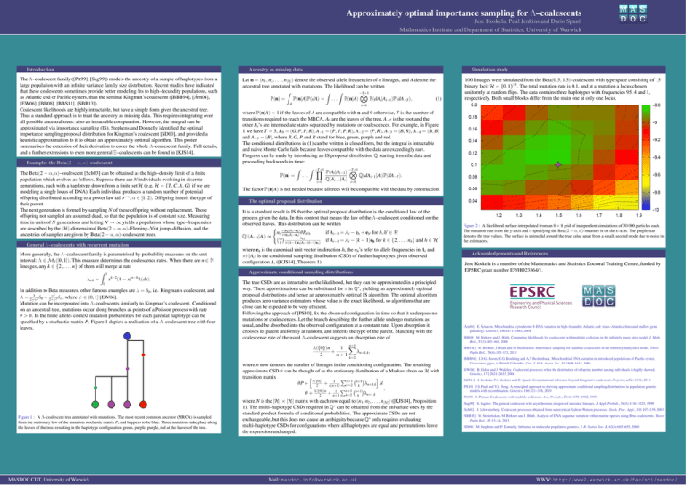
100 lineages were simulated from the Beta(0.5, 1.5)–coalescent with type space consisting of 15
binary loci: H = {0, 1}15. The total mutation rate is 0.1, and at a mutation a locus chosen
uniformly at random flips. The data contains three haplotypes with frequencies 95, 4 and 1,
respectively. Both small blocks differ from the main one at only one locus.
i=0
Λ({0})n
1 X
+
λn+1,k ,
2
n+1
Figure 1 : A Λ–coalescent tree annotated with mutations. The most recent common ancestor (MRCA) is sampled
from the stationary law of the mutation stochastic matrix P, and happens to be blue. Three mutations take place along
the leaves of the tree, resulting in the haplotype configuration green, purple, purple, red at the leaves of the tree.
M A S
D O C
where N is the |H| × |H| matrix with each row equal to (n1, n2, . . . , n|H|) ([KJS14], Proposition
1). The multi–haplotype CSDs required in Q∗ can be obtained from the univariate ones by the
standard product formula of conditional probabilities. The approximate CSDs are not
exchangeable, but this does not cause an ambiguity because Q∗ only requires evaluating
multi–haplotype CSDs for configurations where all haplotypes are equal and permutations leave
the expression unchanged.
Mail: masdoc.info@warwick.ac.uk
Figure 2 : A likelihood surface interpolated from an 8 × 8 grid of independent simulations of 30 000 particles each.
The mutation rate is on the y–axis and α specifying the Beta(2 − α, α)–measure is on the x–axis. The purple star
denotes the true values. The surface is unimodal around the true value apart from a small, second mode due to noise in
the estimators.
Acknowledgements and References
Jere Koskela is a member of the Mathematics and Statistics Doctoral Training Centre, funded by
EPSRC grant number EP/HO23364/1.
[Árn04] E. Árnason. Mitochondrial cytochrome b DNA variation in high–fecundity Atlantic cod: trans–Atlantic clines and shallow gene
genealogy. Genetics, 166:1871–1885, 2004
[BB08] M. Birkner and J. Blath. Computing likelihoods for coalescents with multiple collisions in the infinitely many sites model. J. Math.
Biol., 57(3):435–463, 2008
[BBS11] M. Birkner, J. Blath and M Steinrücken. Importance sampling for Lambda–coalescents in the infinitely many sites model. Theor.
Popln Biol., 79(4):155–173, 2011
[BBB94] J.D.G. Boom, E.G. Boulding and A.T Beckenback. Mitochondrial DNA variation in introduced populations of Pacific oyster,
Crassostrea gigas, in British Columbia. Can. J. Fish. Aquat. Sci., 51:1608–1614, 1994
[EW06] B. Eldon and J. Wakeley. Coalescent processes when the distribution of offspring number among individuals is highly skewed.
Genetics, 172:2621–2633, 2006
[KJS14] J. Koskela, P.A. Jenkins and D. Spanò. Computational inference beyond Kingman’s coalescent. Preprint, arXiv:1311, 2014
[PS10] J.S. Paul and Y.S. Song. A principled approach to deriving approximate conditional sampling distributions in population genetic
models with recombination. Genetics, 186:321–338, 2010
[Pit99] J. Pitman. Coalescents with multiple collisions. Ann. Probab., 27(4):1870–1902, 1999
[Sag99] S. Sagitov. The general coalescent with asynchronous mergers of ancestral lineages. J. Appl. Probab., 36(4):1116–1125, 1999
[Sch03] J. Schweinsberg. Coalescent processes obtained from supercritical Galton–Watson processes. Stoch. Proc. Appl., 106:107–139, 2003
[SBB13] M. Steinrücken, M. Birkner and J. Blath. Analysis of DNA sequence variation within marine species using Beta–coalescents. Theor.
Popln Biol., 87:15–24, 2013
[SD00] M. Stephens and P. Donnelly. Inference in molecular population genetics. J. R. Statist. Soc. B, 62(4):605–655, 2000
WWW: http://www2.warwick.ac.uk/fac/sci/masdoc/