Partial solutions to assignment 2
Math 5080-1, Spring 2011
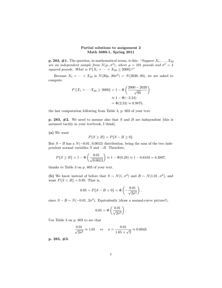
p. 283, #1. The question, in mathematical terms, is this: “Suppose X1 , . . . , X20
are an independent sample from N (µ , σ 2 ), where µ = 101 pounds and σ 2 = 4
squared pounds. What is P {X1 + · · · + X20 ≥ 2000}?”
Because X1 + · · · + X20 is N (20µ , 20σ 2 ) = N (2020 , 80), we are asked to
compute
2000 − 2020
√
P {X1 + · · · X20 ≥ 2000} = 1 − Φ
80
≈ 1 − Φ(−2.24)
= Φ(2.24) ≈ 0.9875,
the last computation following from Table 3, p. 603 of your text.
p. 283, #2. We need to assume also that S and B are independent [this is
assumed tacitly in your textbook, I think].
(a) We want
P {S ≥ B} = P {S − B ≥ 0}.
But S − B has a N (−0.01 , 0.0013) distribution, being the sum of the two independent normal variables S and −B. Therefore,
0.01
P {S ≥ B} = 1 − Φ √
≈ 1 − Φ(0.28) ≈ 1 − 0.6103 = 0.3897,
0.0013
thanks to Table 3 on p. 603 of your text.
(b) We know instead of before that S ∼ N (1 , σ 2 ) and B ∼ N (1.01 , σ 2 ), and
want P {S < B} = 0.95. That is,
0.01
0.95 = P {S − B < 0} = Φ − √
,
2σ 2
since S − B ∼ N (−0.01 , 2σ 2 ). Equivalently (draw a normal-curve picture!),
0.01
0.05 = Φ √
.
2σ 2
Use Table 3 on p. 603 to see that
0.01
√
≈ 1.65
2σ 2
⇔
σ=
p. 283, #3.
1
0.01
√ ≈ 0.0043.
1.65 × 2
(a) We know that
E(X̄) = µ and E(S 2 ) = σ 2 .
Therefore,
E 2X̄ − 5S 2 = 2µ − 5σ 2 .
Now we write things in terms of U and W :
X̄ =
U
,
n
and owing to (8.2.8) on page 266,
S2 =
W − n1 U 2
nW − U 2
=
.
n−1
n(n − 1)
Therefore,



E


5nW − 5U 2
2U
−
n
n(n − 1)
|
{z
}


 = 2µ − 5σ 2 .

an unbiased estimator of 2µ − 5σ 2
(b) Note that E(X12 ) = · · · = E(Xn2 ) = σ 2 +µ2 . Therefore, E(W ) = n(σ 2 +µ2 );
that is, E(W/n) = σ 2 + µ2 . Consequently, W/n is an unbiased estimator of
σ 2 + µ2 .
(c) Note that every Yj takes only two values: 1 [with probability P {X1 ≤
c} = FX (c)] and 0 [with probability 1 − FX (c)]. Therefore, E(Yj ) = FX (c).
This implies that every Yj is an unbiased estimator of FX (c). A more sensible
unbiased estimator can be formed by averaging the Yj ’s:


n
n
X
1
1X
E
Yj  =
E(Yj ) = FX (c).
n j=1
n j=1
Pn
Therefore, n1 j=1 Yj is also an unbiased estimator of FX (c). Although the
following is not a part of the problem, it would be good to ask it: Why is the
average of Y1 , . . . , Yn a better estimate than any one of them? Check that
Var(Y1 ) = · · · = Var(Yn ) = FX (c) {1 − FX (c)} ,
but

n
X
FX (c){1 − FX (c)}
1
Yj  =
,
Var 
n j=1
n

Pn
and this is small when n is large. Therefore, if n is large then n1 j=1 Yj is, with
high probability, close to its expectation FX (c). Whereas the probability that
2
Y1 [say] is within units of FX (c) is some fixed amount and cannot be made
smaller by taking large samples.
p. 283, #4. We compute the joint pdf of (Y1 , Y2 ). First, using calculus
variables, if y1 = x1 + x2 and y2 = x1 − x2 , then
x1 =
y1 + y2
2
and x2 =
And the Jacobian is obtained from


∂x1 ∂x1
1
 ∂y1 ∂y2 
2


J = det 
 = det 
 ∂x
1
∂x2 
2
2
∂y1 ∂y2
y1 − y2
.
2
1
2

 = −1.
2
1
−2
Therefore,
fY1 ,Y2 (y1 , y2 ) = fX1 ,X2 (x1 , x2 )|J|
2
2
2
2 1
1
1
=√
e−(x1 −µ) /(2σ ) √
e−(x2 −µ) /(2σ )
2
2πσ
2πσ
2
2
(x1 − µ) + (x2 − µ)
1
exp −
=
4πσ 2
2σ 2
2
x1 − 2(x1 + x2 )µ + x22 + 2µ2
1
exp
−
=
.
4πσ 2
2σ 2
Now we substitute:
x21 =
y1 + y2
2
2
=
y12 + 2y1 y2 + y22
;
4
x1 + x2 = y1 ;
2
y1 − y2
y 2 − 2y1 y2 + y22
2
x2 =
.
= 1
2
4
Therefore,
x21 − 2(x1 + x2 )µ + x22 + 2µ2 =
y12 − 4µy1 + 4µ2 + y22
(y1 − 2µ)2
y2
=
+ 2.
2
2
2
Plug to find that
1
(y1 − 2µ)2
y22
fY1 ,Y2 (y1 , y2 ) =
exp −
exp − 2 .
4πσ 2
4σ 2
4σ
Therefore, fY1 ,Y2 (y1 , y2 ) can be written as h1 (y1 )h2 (y2 ), which is to say that Y1
and Y2 are independent. Our general theory tells us that Y1 ∼ N (2µ , 2σ 2 ) and
Y2 ∼ N (0 , 2σ 2 ) as well [or you can do a little more algebra and obtain this from
the previous displayed equation].
3