Lecture 12
Let us give several more examples of finding sufficient statistics.
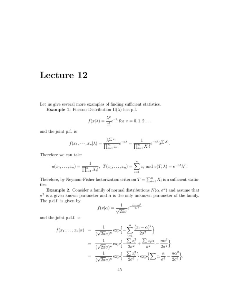
Example 1. Poisson Distribution Π(λ) has p.f.
f (x|λ) =
λx −λ
e for x = 0, 1, 2, . . .
x!
and the joint p.f. is
P
λ
f (x1 , · · · , xn |λ) = Qn
xi
i=1 xi !
Therefore we can take
u(x1 , . . . , xn ) = Qn
1
i=1 Xi !
e−nλ = Qn
, T (x1 , . . . , xn ) =
1
i=1 Xi !
n
X
e−nλ λ
P
Xi
.
xi and v(T, λ) = e−nλ λT .
i=1
P
Therefore, by Neyman-Fisher factorization criterion T = ni=1 Xi is a sufficient statistics.
Example 2. Consider a family of normal distributions N (α, σ 2 ) and assume that
σ 2 is a given known parameter and α is the only unknown parameter of the family.
The p.d.f. is given by
(x−α)2
1
f (x|α) = √
e− 2σ2
2πσ
and the joint p.d.f. is
n
n X
(xi − α)2 o
1
f (x1 , . . . , xn |α) = √
exp −
2σ 2
( 2πσ)n
i=1
n P x2 P x α nα2 o
1
i
i
= √
exp −
+
− 2
2
2
n
2σ
σ
2σ
( 2πσ)
P 2o
n
n
X α
xi
nα2 o
1
exp −
exp
xi 2 − 2 .
= √
2σ 2
σ
2σ
( 2πσ)n
45
46
LECTURE 12.
If we take T =
Pn
i=1
Xi ,
n α
n P x2 o
nα2 o
1
i
and
v(T,
α)
=
exp
T
,
−
u(x1 , . . . , xn ) = √
exp −
2σ 2
σ2
2σ 2
( 2πσ)n
then Neyman-Fisher criterion proves that T is a sufficient statistics.
12.1
Jointly sufficient statistics.
Consider
T1 = T1 (X1 , · · · , Xn )
T2 = T2 (X1 , · · · , Xn )
···
Tk = Tk (X1 , · · · , Xn )







- functions of the sample (X1 , · · · , Xn ).
Very similarly to the case when we have only one function T, a vector (T1 , · · · , Tk ) is
called jointly sufficient statistics if the distribution of the sample given T ’s
θ (X1 , . . . , Xn |T1 , . . . , Tk )
does not depend on θ. The Neyman-Fisher factorization criterion says in this case
that (T1 , . . . , Tk ) is jointly sufficient if and only if
f (x1 , . . . , xn |θ) = u(x1 , . . . , xn )v(T1 , . . . , Tk , θ).
The proof goes without changes.
Example 1. Let us consider a family of normal distributions N (α, σ 2 ), only now
both α and σ 2 are unknown. Since the joint p.d.f.
n P x2 P x α nα2 o
1
i
i
2
f (x1 , . . . , xn |α, σ ) = √
exp −
+
− 2
2
2
n
2σ
σ
2σ
( 2πσ)
is a function of
T1 =
n
X
i=1
Xi and T2 =
n
X
Xi2 ,
i=1
by Neyman-Fisher criterion (T1 , T2 ) is jointly sufficient.
Example 2. Let us consider a uniform distribution U [a, b] on the interval [a, b]
where both end points are unknown. The p.d.f. is
1
, x ∈ [a, b],
b−a
f (x|a, b) =
0,
otherwise.
47
LECTURE 12.
The joint p.d.f. is
1
I(x1 ∈ [a, b]) × . . . × I(xn ∈ [a, b])
(b − a)n
1
I(xmin ∈ [a, b]) × I(xmax ∈ [a, b]).
=
(b − a)n
f (x1 , · · · , xn |a, b) =
The indicator functions make the product equal to 0 if at least one of the points falls
out of the range [a, b] or, equivalently, if either the minimum xmin = min(x1 , . . . , xn )
or maximum xmax = max(x1 , . . . , xn ) falls out of [a, b]. Clearly, if we take
T1 = max(X1 , . . . , Xn ) and T2 = min(X1 , . . . , Xn )
then (T1 , T2 ) is jointly sufficient by Neyman-Fisher factorization criterion.
Sufficient statistics:
• Gives a way of compressing information about underlying parameter θ.
• Gives a way of improving estimator using sufficient statistic (which takes us to
our next topic).
12.2
Improving estimators using sufficient statistics. Rao-Blackwell theorem.
(Textbook, Section 6.9)
Consider δ = δ(X1 , · · · , Xn ) - some estimator of unknown parameter θ0 , which
corresponds to a true distribution θ0 of the data. Suppose that we have a sufficient
statistics T = T (X1 , · · · , Xn ). (T can also be a vector of jointly sufficient statistics.)
One possible natural measure of the quality of the estimator δ is the quantity
θ0 (δ(X1 , . . . , Xn )
− θ 0 )2
which is an average squared deviation of the estimator from the parameter θ0 .
Consider a new estimator of θ0 given by
δ 0 (X1 , . . . , Xn ) =
θ0 (δ(X1 , . . . , Xn )|T (X1 , . . . , Xn )).
Question: why doesn’t δ 0 depend on θ0 even though formally the right hand side
depends on θ0 ?
Recall that this conditional expectation is the expectation of δ(x1 , . . . , xn ) with
respect to conditional distribution
θ0 (X1 , . . . , Xn |T ).
48
LECTURE 12.
Since T is sufficient, by definition, this conditional distribution does not depend on
the unknown parameter θ0 and as a result δ 0 doesn’t depend on θ0 . This point is
important, since the estimate can not depend on the unknown parameter, we should
be able to compute it using only the data.
Another important point is that the conditional distribution and, therefore, the
conditional expectation depend only on T, which means that our new estimate δ 0
actually depends on the data only through T, i.e. δ 0 = δ 0 (T ).
Theorem. (Rao-Blackwell) We have,
θ0 (δ
0
− θ 0 )2 ≤
− θ 0 )2
θ0 (δ
Proof. Given random variable X and Y, recall from probability theory that
{ (X|Y )}.
X=
Clearly, it we can prove that
θ0 ((δ
0
− θ0 )2 |T ) ≤
θ0 ((δ
then averaging both side will prove the Theorem.
First, consider the left hand side. Since δ 0 =
θ0 ((δ
0
− θ0 )2 |T ) =
θ0 ((
− θ0 )2 |T )
θ0 (δ|T ),
θ0 (δ|T )
− θ0 )2 |T ) = . . .
Since ( θ0 (δ|T ) − θ0 )2 is already a function of T we can remove the conditional
expectation given T and continue
... = (
θ0 (δ|T )
− θ 0 )2 = (
θ0 (δ|T ))
2
− 2θ0
θ0 (δ|T )
+ θ02 .
Next, we consider the right hand side. Squaring out we get,
θ0 ((δ
− θ0 )2 |T ) = (
θ0 (δ
2
|T )) − 2θ0
θ0 (δ|T )
+ θ02 .
Therefore, to prove that LHS ≤ RHS, we need to show that
(
θ0 (δ|T ))
2
≤
θ0 (δ
2
|T ).
But this is the same as
0≤
θ0 (δ
2
|T ) − (
θ0 (δ|T ))
2
= Varθ0 (δ|T )
which is obvious since the variance Varθ0 (δ|T ) is always positive.