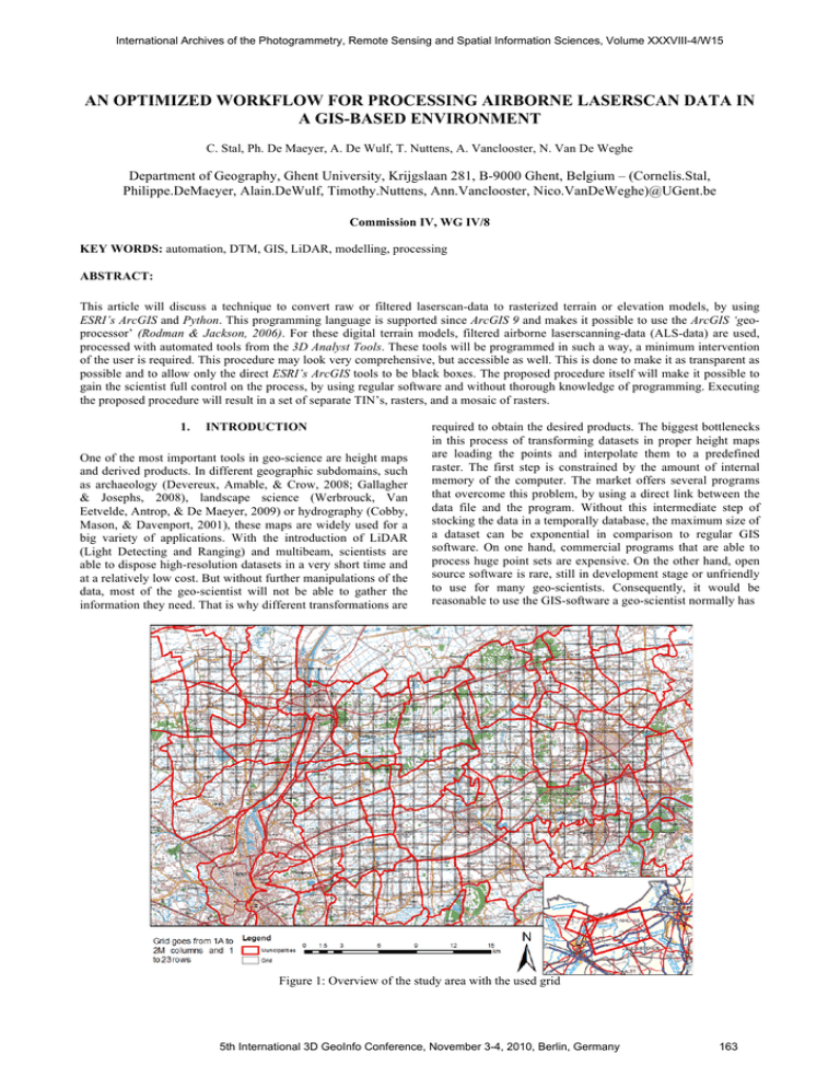
International Archives of the Photogrammetry, Remote Sensing and Spatial Information Sciences, Volume XXXVIII-4/W15
AN OPTIMIZED WORKFLOW FOR PROCESSING AIRBORNE LASERSCAN DATA IN
A GIS-BASED ENVIRONMENT
C. Stal, Ph. De Maeyer, A. De Wulf, T. Nuttens, A. Vanclooster, N. Van De Weghe
Department of Geography, Ghent University, Krijgslaan 281, B-9000 Ghent, Belgium – (Cornelis.Stal,
Philippe.DeMaeyer, Alain.DeWulf, Timothy.Nuttens, Ann.Vanclooster, Nico.VanDeWeghe)@UGent.be
Commission IV, WG IV/8
KEY WORDS: automation, DTM, GIS, LiDAR, modelling, processing
ABSTRACT:
This article will discuss a technique to convert raw or filtered laserscan-data to rasterized terrain or elevation models, by using
ESRI’s ArcGIS and Python. This programming language is supported since ArcGIS 9 and makes it possible to use the ArcGIS ‘geoprocessor’ (Rodman & Jackson, 2006). For these digital terrain models, filtered airborne laserscanning-data (ALS-data) are used,
processed with automated tools from the 3D Analyst Tools. These tools will be programmed in such a way, a minimum intervention
of the user is required. This procedure may look very comprehensive, but accessible as well. This is done to make it as transparent as
possible and to allow only the direct ESRI’s ArcGIS tools to be black boxes. The proposed procedure itself will make it possible to
gain the scientist full control on the process, by using regular software and without thorough knowledge of programming. Executing
the proposed procedure will result in a set of separate TIN’s, rasters, and a mosaic of rasters.
1.
INTRODUCTION
One of the most important tools in geo-science are height maps
and derived products. In different geographic subdomains, such
as archaeology (Devereux, Amable, & Crow, 2008; Gallagher
& Josephs, 2008), landscape science (Werbrouck, Van
Eetvelde, Antrop, & De Maeyer, 2009) or hydrography (Cobby,
Mason, & Davenport, 2001), these maps are widely used for a
big variety of applications. With the introduction of LiDAR
(Light Detecting and Ranging) and multibeam, scientists are
able to dispose high-resolution datasets in a very short time and
at a relatively low cost. But without further manipulations of the
data, most of the geo-scientist will not be able to gather the
information they need. That is why different transformations are
required to obtain the desired products. The biggest bottlenecks
in this process of transforming datasets in proper height maps
are loading the points and interpolate them to a predefined
raster. The first step is constrained by the amount of internal
memory of the computer. The market offers several programs
that overcome this problem, by using a direct link between the
data file and the program. Without this intermediate step of
stocking the data in a temporally database, the maximum size of
a dataset can be exponential in comparison to regular GIS
software. On one hand, commercial programs that are able to
process huge point sets are expensive. On the other hand, open
source software is rare, still in development stage or unfriendly
to use for many geo-scientists. Consequently, it would be
reasonable to use the GIS-software a geo-scientist normally has
Figure 1: Overview of the study area with the used grid
5th International 3D GeoInfo Conference, November 3-4, 2010, Berlin, Germany
163
International Archives of the Photogrammetry, Remote Sensing and Spatial Information Sciences, Volume XXXVIII-4/W15
and develop tools for this software to obtain comparable results
of specialized software packages.
In other words, it will be shown that a GIS-software can be used
to process LiDAR data The performance of processing and
analysing rasterized LiDAR data in a GIS is shown to be good
(Brovelli, Cannata, & Longoni, 2002; Hewett, 2005), which is
about the automatic feature extraction out of these data, and will
not be discussed here.
The entire process is illustrated in a flowchart, which can be
found in the next paragraph. This flowchart is developed on
behalf of a landscape research in the Flemish region of the
“Waasland” (Werbrouck, et al., 2009), visualized in figure 1.
On behalf of this article, airborne LiDAR-data with a regular
ASCII format is assumed. Other formats, like the binary .lasformat will not be used and discussed. In section 2, a short
overview will be given about the used program and data. The
entire workflow is summarized in section 3. The preparation of
this data for the purposed workflow is given in section 4. After
this preparation, the raw dataset will be divided over an external
grid (section 5) and interpolated (section 6). A conclusion will
be given in section 7.
2.
OVERVIEW OF THE USED PROGRAMS AND
TOOLS
ESRI’s ArcGIS is, in principle, not meant to process huge point
clouds, and special tools or add-ins for this GIS-environment do
not exist. Even though ‘multipoints’ are introduced in the
ArcGIS 9.3 version, the performance of analyzing and
processing large datasets is low. The ‘multipoint’ is a new
feature class in ArcGIS to store multiple points, where each
record contains a sub-collection of points, instead of storing
each point in a single record. There are several programs and
extensions from other vendors, which complement ArcGIS and
make it possible to read and process big datasets. These tools
are both commercial software (like LP360) and open source
(like GISLiDARTools). The latter is only able to read datasets
with the .las-format (version 1.0, www.lasformat.org). Since the
Flemish Agency for Geographic Information (AGIV) does not
use this binary format, but regular x,y,z-files (AGIV, 2008),
another conversion is needed to use this .las-format. This can be
done by the free LASTools, developed by (Isenburg &
Shewchuk, 2010) where straight conversion from x,y,z-files via
point primitives to rasters is preferred. In this article, ESRI’s
ArcGIS (more specific: ArcGIS 9.3 Desktop) is used, with the
3D Analyst Tools-license and Python. The fact that only these
tools are used is the strength of the proposed method, because of
the wide availability. The execution of the procedures will be
discussed, with special interest to the used commands and the
required parameters. Optional parameters will only be discussed
when relevant. The procedures are figured in a flowchart,
presented in figure 2. More information about the used Pythonscripts can easily be found for each operator in the ArcGIS Help
and on the program’s website (webhelp.esri.com).
Many tasks can be automated in ArcGIS. On one hand, ArcGIS
can be extended by writing scripts in, for example, VBA. This is
a very common way to make new tools or automate and
combine existing tools. It is also possible to use the ArcGIS
Model Builder, but the possibility to loop operations is limited
(for example: the query “get all ascii-files in a given directory
and convert them to shapefiles” is not possible by the Model
Builder). On the other hand, it is more powerful to call tools in
Python, an 'easy-to-learn imperative, object oriented
programming language' (Butler, 2004). Python is an open
source language, with human readable code, a very small
interpreter and straightforward and a wide available libraries
and dependencies. This increases the exchangeability and the
possibility to modify code by more users (Rodman & Jackson,
2006). By linking ArcGIS tools to ‘lists’, and by working with
automatically determined parameters in a loop, a lot of
procedures can be executed with minimal user intervention.
Especially for tasks, that have to be executed many times,
Python is advisable. Besides the standard library of Python,
objects and modules can be imported from ArcGIS, the so called
ArcObjects. The user is able to find the tool’s declaration in the
help, within ArcGIS. In the Python IDE, and scripts can be
modified and supplemented if needed. When ready, they are
saved as .py-files. These files can be executed in the IDE itself
or the OS command prompt.
Figure 2: Flowchart of the rasterization of filtered LiDAR-data
164
5th International 3D GeoInfo Conference, November 3-4, 2010, Berlin, Germany
International Archives of the Photogrammetry, Remote Sensing and Spatial Information Sciences, Volume XXXVIII-4/W15
3. FLOWCHART AND PROCEDURE OVERVIEW
As demonstrated in the flowchart (figure 2), the raw data of the
AGIV contains, besides metadata, three datasets. To construct a
DTM, only the ground data (in ASCII-format) are converted to
a shapefile by the AsciiToFeatureclass_3D command.
Based on the geometry of the study area, a grid and empty
TIN’s are constructed and the shapefiles, containing all points
per flight strip, are clipped. Then, all points within a flight strip
(section) are split, based on this grid. Points, located in one cell
from different flight strips are merged together. This point sets
are used to fill the empty TIN’s, one for each cell, resulting in
the first useful product of this procedure. For each cell, a raster
set, containing interpolated height values can be constructed by
converting the TIN’s. If required, a mosaic can be made by
merging this rasters. A more detailed exposition is given in this
paper.
4.
Figure 3: Flight strips, core area and its neighboring areas
PREPARATION
Before any ArcGIS-process can be programmed in Python, a
‘geo-processor’, in the code samples referred as ‘gp’ in the
scripts, needs to be declared. This ‘geo-processor’ makes it
possible to call every ArcGIS-operator. Therefore, the
processor-module needs to be imported and a new ‘geoprocessor’ needs to be made. The syntax may look like this:
# Create a GeoProcessor
import arcgisscripting
gp = arcgisscripting.create()
A lot of tools in ArcGIS require specific extensions. The
availability of different tools depends on the used license. In
the presented work, the 3D Analyst Tools license is required.
These tools need to be called explicitly in Python as well. Please
note that some tools may be available in different toolsets, and
can be called in different ways. Calling the 3D Analyst Tools
can be done by writing:
# Call the 3D Analyst Tools extension
gp.CheckOutExtension ("3D")
Based on practical experience and tests, it must be concluded
that ArcGIS is not powerful enough to interpolate huge point
clouds, using Kriging or Inverse Distance Weight (Prathumchai
& Samarakoon, 2006). The raw datasets, delivered by the
AGIV, have a point density of approximately 1 point per 4 m2,
randomly divided. Making a raster with a 2 meter resolution by
simple linear interpolation is sufficient for this operation. This
density means that a dataset, covering 1 km2, contains about
250,000 points, which can easily be managed by common
processing software and ArcGIS. The dataset that needs to be
processed covers an area of 600 km2, resulting in about 150
million points. It is hardly possible to process this amount of
points using current personal computers with regular GISsoftware. The entire area shall be divided in squared sectors of
1.44 km2. This means a core area of 1 km2, and an overlap with
its neighbours of 100 meters on each side of the cell. Bigger
core areas will increase the burden of internal memory and
decrease the performance of the procedure. Furthermore,
separate rasters of 1 km2 seems to have a reasonable size for
morphological research on micro scale. The division will be
defined in a shapefile, where it should be described with
polygons. Each polygon contains an index as well, which will
be used to call a specific area that has to be processed. The
concept of this indexation is illustrated in figure 3.
5.
DIVISION OF THE RAW DATASET WITHIN AN
EXTERNAL REGULAR GRID
5.1 Supplied data
Besides the already mentioned raw point cloud, in ASCII-file
format, the AGIV also supplies metadata and a shapefile
describing the supplied area. Each file contains an (x,y,z)
description of each point. For every flight strip, a compressed
folder is made, containing both ground- and non-ground points
(respectively .grd and .veg files). In this case, only the ground
points will be used, so these files will be decompressed and
placed in a separate folder.
5.2 Converting to shapefiles
Before the filtered ALS-data can be used in ArcGIS, they need
to be converted to shapefiles. To speed up the process,
‘multipoints’ will be chosen as feature class type. As said
before, this feature class type stores every point in a massive
point set, so independent points cannot be called. The
advantages of this type are that every tool in the program can
still be used, even faster than using the regular point geometry,
and the size of the data is significant smaller than a regular
shapefile containing the same point data. The conversion will be
done by the ‘ASCII to Feature Class’-tool. The file to convert,
the feature class type and the input format need to be called.
AGIV’s ALS-data always have the “XYZ” input format.
Finally, the name of the exported file is given, together with the
feature class type. For ALS-data, the user can choose between
‘point’ and ‘multipoint’.
# Create a shapefile by converting an
ASCII-gridfile
gp.asciitofeatureclass_3D(<INPUT>,
”XYZ”,
<OUTPUT> + “.shp”, “Multipoint”)
After this conversion, only the points, located within the
research area are used. Separating these points from the points
outside this area can be done by the ‘clip’-command. This
command can be called by the following script:
# Get the points, locating within the study
area
gp.clip(<POINTSET>, <STUDY AREA>, <OUTPUT>,
“POINT”)
5th International 3D GeoInfo Conference, November 3-4, 2010, Berlin, Germany
165
International Archives of the Photogrammetry, Remote Sensing and Spatial Information Sciences, Volume XXXVIII-4/W15
5.3 Division of the data by a grid
The data shall be divided by a grid, which covers the entire
study area. This grid has been discussed in section 3 and has a
cell size of 1200 by 1200 meter. In the phase where the TINs
are constructed, no other points than the points within a specific
cell are used and there is no relation with other points in
neighbouring cells, so overlapping zones are needed when a
mosaic is made of several rasters. Without this overlap, the
merged rasters would have gaps along the borders of each cell.
These gaps will have the same size as the resolution of the
model. Therefore, it is of great importance that the cells have an
overlap with their neighbours. During the linear interpolation of
the TIN’s, the rasters are not supplemented by extrapolated
data, or data from other areas. When the TIN’s are converted to
rasters, and these rasters have to be merges (mosaic), the height
values of the overlapping areas can be averaged, blend,
minimized, maximum.
A folder is made for every dataset, where the divided shapefiles
shall be stored. Making a new folder in Python can be done by
the mkdir-command, after importing the os-module. The basis
of the split-operation is the grid that has been made. Each
element of this grid will be placed in a list, that will be called by
the iterator. Every new shapefile gets the name of the grid cell,
containing the data.
# Create new shapefiles, based on the
location and index
gp.split(<FILE_IN>,
<INDEX>,
“Index”,
<TARGET WORKSPACE>)
This command requires the flight strip and a split feature,
accompanied with the index of a specific cell. The target
workspace is the location where the split features will be stored.
After splitting the strips by the squared index-cells, the
shapefiles from different flight strips, located in the same indexcell have to be merged again. A loop is programmed to search
for every shapefile available per cell having the reference to this
specific index-cell in the grid. When a file is found, its location
will be stored in a string <FILELIST>. Every file in this
string will be merged to a new shapefile, having the name of the
regarding index <FILE_OUT>.
in this intermediate step, is that TINs can be a useful product for
other research.
6.2 Conversion via TIN
In ArcGIS, the creation of a TIN for a specific dataset, is
performed in two steps. In the first step, an empty TIN is
created. This TIN will be filled in the second step with the
desired dataset. Optionally, other shapefiles, containing break
lines, can be added to improve the quality of the model (Weng,
2002). Especially for areas with complex topography, this could
be useful. In this case, no break lines are available.
# Create an empty TIN
gp.createtin_3d(<TINNAME>)
# Edit the created TIN, by allocating the
shapefiles
gp.edittin_3d(<TINNAME>,
<SHAPEFILE>,
"Shape", "#", "masspoints", "true")
A TIN can be converted to a raster, by using the ‘Convert TIN
to Raster’-tool. The parameters this tool needs, are the name of
the TIN, that needs to be converted and the name of the new
raster to be made. Other parameters are optional, but interesting
to mention. The datatype determines whether the raster must
contain integer or floating values. The resolution and z-factor
determine respectively the cell size and multiplication factor for
the height values. After using this tool, a DTM is created,
consisting of a raster, which represents every available height
values.
# Convert a TIN to a new Raster
gp.tinraster_3d(<TINNAME>,
<OUTNAME>,
<TYPE>, <METHOD>, <RES>, <Z-FACTOR>)
The final raster set is ready for further analysis by the specialist
that needs the final model. It is possible to make a mosaic of all
rasters. Once again, Python is recommended to speed up this
process. An example of this raster is illustrated in figure 4.
# Merge shapefiles, containing parts of an
index to a new shapefile
gp.merge(<FILELIST>, <FILE_OUT>)
6.
CONVERTING SHAPEFILES TO A DIGITAL
TERRAIN MODEL
6.1 Overview
So far, only thorough division of the point clouds has taken
place. No original data is lost in the entire study-area. In the
next step, random-divided points will be interpolated to a
regular grid and finally, to a raster representing height-values.
Initially, every shapefile, representing one specific cell with one
index in the study-area, is converted to a TIN. Thereafter, a
regular grid is interpolated for each TIN, locating in an indexcell and its overlapping zones. Since the original data has an
average point density of one point per 4 m2, a final resolution of
2 meter is chosen. By choosing this resolution, a linear
interpolation of the triangles in the TIN is justified. The
difference of this method, Inverse Distance Weight (IDW)
(which is used by the AGIV) or Kriging is small (Droj, 2008;
Siska & Hung, 2001). Another problem with the IDW and
Kriging interpolation methods, is that it takes a very long time
to make the required calculations in ArcGIS, even when Python
is used to automate the process. Another profit of creating TINs
166
Figure 4: Example of a converted and merged height raster
5th International 3D GeoInfo Conference, November 3-4, 2010, Berlin, Germany
International Archives of the Photogrammetry, Remote Sensing and Spatial Information Sciences, Volume XXXVIII-4/W15
7.
CONCLUSION
The importance of LiDAR-data is growing for many geo-related
sciences since a few years. This development emphasize the
importance of accessible tools to process this data. In this
article, a workflow is optimized to process airbone LiDAR data.
In this process, ESRI’s ArcMap is used and this GIS
environment is extended by implemented tools in Python. Many
tools from ArcGIS are used by calling them in a straightforward
way, in order to transform huge point clouds to regular grids.
First, the ASCII-files are converted to the ESRI’s shapefiles,
and then, operators like ‘split’, ‘clip’ and ‘merge’ are used. The
models and the interpolation to get them relies on TINs. The
advantage of this method is that no further software is required
and its accessibility for geo-scientist, not familiar in
informatics.
REFERENCES
AGIV (2008). Metadataset: DHM Vlaanderen, LIDAR
hoogtepunten - brondata. metadata.agiv.be. Retrieved from
http://metadata.agiv.be/Details.aspx?fileIdentifier=4a23f2e7aadd-4321-82d9-50fcd35fa856
Brovelli, M. A., Cannata, M., & Longoni, U. M. (2002).
Managing and processing Lidar data within GRASS. Paper
presented at the Proceedings of the Open Souirce GIS - Grass
users conference, 11-13 september 2002, Trento, Italië.
Butler, H. (2004). A Guide to the Python Universe for ESRI
Users. Paper presented at the Annual ESRI International
Conference, San Diego, California, USA.
Cobby, D. M., Mason, D. C., & Davenport, I. J. (2001). Image
processing of airborne scanning laser altimetry data for
imporved river flood modelling. ISPRS Journal of
Photogrammetry & Remote Sensing 56, 121-138.
Droj, G. (2008). Improving the Accuracy of Digital Terrain
Models. Studia Universitatis Babes-Bolyai: Series Informatica,
LIII(1), 65-72.
Gallagher, J. M., & Josephs, R. L. (2008). Using LiDAR to
Detect Cultural Resources in a Forested Environment: an
Example from Isle Royale National Park, Michigan, USA.
Archeological Prospection, 15, 187-206.
Hewett, M. (2005). Automating Feature Extraction with the
ArcGIS Spatial Analyst Extension. Paper presented at the
Annual ESRI International Conference, San Diego, California,
USA.
Isenburg, M., & Shewchuk, J. (2010). LAStools (Version 1.2).
http://www.cs.unc.edu/~isenburg/lastools/.
Prathumchai, K., & Samarakoon, L. (2006). Elevation Surface
Interpolation of Point Data Using Different Techniques - a GIS
Approach. Paper presented at the Asian Association on Remote
Sensing.
Rodman, L., & Jackson, J. (2006). Creating Stand-Alone
Spatially Enabled Python Applications Using the ArgGIS
Geoprocessor. Paper presented at the Annual ESRI
International Conference.
Siska, P., P., & Hung, I.-K. (2001). Assessment of Kriging
Accuracy in the GIS Environment. Paper presented at the
Annual ESRI International Conference.
Weng, Q. (2002). Quantifying Uncertainty of Digital Elevation
Models. Paper presented at the International Symposium on
Spatial Data Handling (SDH).
Werbrouck, I., Van Eetvelde, V., Antrop, M., & De Maeyer, P.
(2009). Integrating Historical Maps and LiDAR Elevation Data
for Landscape Reconstruction: a case study in Flanders
(Belgium). Paper presented at the European Landscapes in
Transformation; Challenges for Landscape Ecology and
Management, Salzburg, Austria.
Devereux, B. J., Amable, G. S., & Crow, P. (2008).
Visualisation of LiDAR Terrain Models for Archeological
Feature Detection. Antiquity, 82, 470-479.
5th International 3D GeoInfo Conference, November 3-4, 2010, Berlin, Germany
167