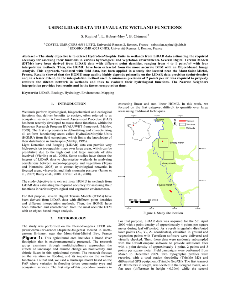
USING LIDAR DATA TO EVALUATE WETLAND FUNCTIONS
S. Rapinel 1, L. Hubert-Moy 1, B. Clément 2
1
COSTEL UMR CNRS 6554 LETG, Université Rennes 2, Rennes, France - sebastien.rapinel@uhb.fr
2
ECOBIO UMR 6553 CNRS, Université Rennes 1, Rennes, France
Abstract – The study objective is to extract HydroGeoMorphic Units in wetlands from LiDAR data estimating the required
accuracy for assessing their functions in various hydrological and vegetation environments. Several Digital Terrain Models
(DTMs) have been derived from LiDAR data with different point densities, ranging from 4 to 1 point/m² with four
interpolation methods. Then, the HGMU have been extracted from the more accurate DTM with an Object-based Image
Analysis. This approach, validated with field data, has been applied in a study site located near the Mont-Saint-Michel,
France. Results showed that the HGMU map quality highly depends primarily on the LIDAR data precision (point-density)
and, in a lesser extent, on the interpolation method used. A minimum precision of 2 points per m² was required to properly
restitute the ditches network in wetlands and thus to evaluate their hydrological functions. The Nearest Neighbors
interpolation provides best results and in the fastest computation time.
Keywords: LiDAR, Ecology, Hydrology, Environment, Mapping
1.
INTRODUCTION
Wetlands perform hydrological, biogeochemical and ecological
functions that deliver benefits to society, often referred to as
ecosystem services. A Functional Assessment Procedure (FAP)
has been recently developed to assess these functions, within the
European Research Program EVALUWET framework (Maltby,
2009). The first step consists in delimitating and characterizing
all uniform functioning areas called HydroGeoMorphic Units
(HGMU) from field campaigns, which limits the knowledge of
their distribution in landscapes (Matlby, 1996).
Light Detection and Ranging (LiDAR) data can provide very
high-precision topographic maps over large areas, which can be
prohibitive due to the high cost and large amounts of data
involved (Vierling et al., 2008). Some studies have shown the
interest of LiDAR data to characterize wetlands in analyzing
correlations between micro-topography and vegetation (Toyra
and Pietroniro, 2005) or to extract hydrological networks in
forested areas, vineyards, and high mountain pastures (James et
al., 2007; Bailly et al., 2008 ; Cavalli et al., 2008).
extracting linear and non linear HGMU. In this work, we
focused on the first category, difficult to quantify over large
areas using traditional techniques.
The study objective is to extract linear HGMU in wetlands from
LiDAR data estimating the required accuracy for assessing their
functions in various hydrological and vegetation environments.
For that purpose, several Digital Terrain Models (DTMs) have
been derived from LiDAR data with different point densities
and different interpolation methods. Then, the HGMU have
been extracted and characterized from the most accurate DTM
with an object-based image analysis.
2.
Figure 1. Study site location
METHODOLOGY
The study was performed on the Pleine-Fougères LTER site
(www.caren.univ-rennes1.fr/pleine-fougeres) located in northeastern Brittany, near the Mont-Saint-Michel Bay, France
(Figure 1). This agricultural area includes a broad river
floodplain that is environnementally protected. The research
group examines through multidisciplinary approaches the
effects of landscape and climate change on biodiversity and
abiotic fluxes in this agricultural system. The research focuses
on the variation in flooding and its impacts on the wetland
functions. To that end, we used a landscape model based on the
FAP where variation in flooding drives community type and
ecosystem services. The first step of this procedure consists in
For that purpose, LiDAR data was acquired for the 5th April
2009 with a point density of approximately 4 points per square
meter during leaf off period. As a result irregularly distributed
laser points (X-, Y-, Z- coordinates), classified in ground and
vegetation points with TerraScan software were delivered and
visually checked. Then, these data were randomly subsampled
with the CloudCompare software to provide additional files
with a point density of approximately 1 point, 2 points and 3
points per square meter. Field campaigns were performed from
March to December 2009. Two topographic profiles were
recorded with a total station theodolite (Trimble M3) and
differential GPS equipment (Trimble GeoXH). The first transect
of 100 meters in length, was located in the Sougeal marsh, on a
flat area (difference in height <0.30m) while the second
transect, located in the Boucey marsh, covers a ditch section of
4 meters length with a deeper slope (difference in height
>0.50m). All field measurements were integrated into a GIS
database. The irregularly dispersed laser points assumed to
correspond to the ground were used to derive high–accuracy
Digital Terrain Models (DTMs) with four interpolation
methods, Nearest Neighbors (NN), Inverse Distance Weighted
(IDW), Spline and ordinary kriging. The set of parameters used
for these calculations is shown in Table A. For the kriging
method, a variogram was calculated for each test area. The
output grid cell datasets were fixed at 0.50 meter. Calculations
were run for the four point densities. Mean elevation differences
between the field-measurements and the LiDAR DTMs were
measured by the Root Mean Square Error (RMSE).
Table A. Interpolations parameters
Interpolation
NN
IDW
Spline
Kriging
Parameters
None
Power=2 ; Search radius=variable with
12 points
Type=tension ; Weight = 0.1 ; Number of
points=12
Sougeal marsh:
Variogram type = Power
Power 1.27 , Length 150, Slope 0.005,
Nugget effect 0.01
Boucey marsh:
Variogram type = Exponential
Scale 0.02 ,Length 30, Nugget effect
0.012
Then, linear HGMU were extracted from the DTM with the
lowest RMSE by an object-oriented approach performed with
an eCognition software package: A line extraction algorithm
was applied on DTM to detect linear objects. Then, primitive
objects were segmented and merged along their main direction.
Finally, linear objects were classified in four classes according
to their depth (Table B). This approach was applied on two
close areas (Test areas) of 25 hectares each within the study site
to evaluate the impact of wooded vegetation on DTM’
accuracy: in the first one, located in the Boucey marsh, ditches
are often bordered by tree-lines, while there are no wooded
hedges in the Aucey marsh. Classification results were validated
with a HGMU field map.
3.
RESULTS AND DISCUSSION
RMSE values of the DTMs calculated for the two transects were
compared for the four interpolation methods and the four
ground-point densities (Table C). On the Sougeal marsh, all
DTMs have the same global RMSE value (0.12 m), whatever
the ground-point density or the interpolation method. On flat
herbaceous meadows, RMSE values decrease by less than
0.05 m.
On the contrary, on flooded areas, where no LiDAR returns
occur because of the presence of open water, RMSE values
increase up to 0.30 m. On the flow ditch located at the Boucey
marsh, RSME values range from 0.12 to 0.27 m. As expected,
best results were obtained with a higher ground-point density.
RSME values significantly increase with a ground point density
of 1 point per m². DTMs derived using the Nearest Neighbors or
the Spline interpolation methods (RMSE: 0.12 m) have a better
accuracy than DTMs derived using the Inverse Distance
Weighted (RMSE: 0.15 m) and the kriging methods (RMSE:
0.19 m). These results confirm a previous study showing the
superiority of the NN interpolation method compared to the
IDW for DTMs derived from high point density datasets (Bater
and Coops, 2009). The comparison between the DTMs profiles
derived from LiDAR data and the field measurements shows
that all DTMs underestimate the ditch depth (
Figure 2). This could be explained by the presence of open
water and dense herbaceous vegetation within the ditch. Figure
2 also highlighted the fact that the DTMs obtained by the NN
interpolation method with a ground-point density of 4 points per
m² best fitted with field measurements. This DTM was therefore
selected for the detection of linear HGMU.
Table C. RMSE values according to the ground-point density
and the interpolation method (in meters)
Interpo
lation
method
NN
IDW
Spline
Kriging
Ground-point density (m²)
Boucey marsh
Sougeal marsh
4
3
2
1
4
3
2
1
0,14 0,12 0,16 0,24 0,12 0,12 0,12 0,12
0,15 0,15 0,14 0,27 0,12 0,12 0,12 0,12
0,14 0,15 0,16 0,24 0,12 0,12 0,12 0,12
0.19 0.20 0.18 0.27 0,12 0,12 0,12 0,12
Table B. Classification scheme of linear HGMU
Linear HGMU
classes
1. Drainage ditch
2. Flow ditch
3. Evacuation
ditch
4. Channel
Characteristic
Depth <20 cm
No variation between ditch’s and adjoining
parcel’s vegetation
Depth <50 cm
Variation between ditch’s and adjoining
parcel’s vegetation
Depth >50 cm
Large variation between ditch’s and
adjoining parcel’s vegetation
Depth >50 cm ; wide > 100 cm
Large variation between ditch’s and
adjoining parcel’s vegetation
Figure 2. Comparison between DTMs derived from LiDAR data
and field measurements on a ditch
The results of the classification performed with the objectoriented approach to extract linear HGM showed significant
accuracy differences between classes (Table D). Channels and
evacuation ditches were better identified than drainage and flow
ditches, because the latter are less deep and wider. On the marsh
Boucey, accuracy levels were lower because of the presence of
hedgerows along the ditches that leads to no LiDAR returns.
This finding is particularly true for drainage ditches, less deep
and with a higher proportion of area covered by tree canopy.
The results also pointed out that all classes were detected with a
very small over detection.
Linear HGMU maps are presented on Figure 3. Almost all
linear HGMU that were not detected by the object-oriented
approach will be successfully mapped by photo-interpretation
techniques.
Table D. Accuracy indicators of the linear HGMU classification
on Aucey and Boucey marshes
fastest computation time, global computing time being less than
10 minutes for a 25-hectares area including DTM generation
and automatic linear HGMU extraction.
Moreover, two limitant factors have been identified for the
mapping of linear HGMU: the presence of open water and
vegetation, even during the leave-off period.
From these
results, the mapping of HGMU is currently carried out on a 650
km² watershed in the Dordogne region with over 8 billions of
LiDAR points in order to evaluate wetland hydrological
functions.
REFERENCES
Detection
(%)
Drainage
ditch
Flow ditch
Evacuation
ditch
Channel
Aucey marsh
Well
Over
detected detected
Boucey marsh
Well
Over
detected detected
56.8
00.9
32.2
03.0
36.9
04.5
58.9
01.6
93.2
00.0
82.2
05.7
95.4
00.0
J. S. Bailly, P. Lagacherie, C. Millier, C. Puech, et P. Kosuth,
“Agrarian landscapes linear features detection from LiDAR:
application to artificial drainage networks,” International
Journal of Remote Sensing, vol. 29, n°. 11, p. 3489-350, 2008.
W. Bater and N. C. Coops, “Evaluating error associated with
lidar-derived DEM interpolation,” Computers & Geosciences,
vol. 35, n°. 2, p. 289-300, 2009.
M. Cavalli, P. Tarolli, L. Marchi and G. Dalla Fontana, “The
effectiveness of airborne LiDAR data in the recognition of
channel-bed morphology,” CATENA, vol. 73, n°. 3, p. 249-260,
2008.
L. A. James, D. G. Watson, and W. F. Hansen, “Using LiDAR
data to map gullies and headwater streams under forest canopy:
South Carolina, USA,” CATENA, vol. 71, n°. 1, p. 132-144,
2007.
E. Maltby, N. Mockler, and R. Mcinnes, “Denitrification rates
in river marginal wetlands and buffer zone management,” in Les
colloques, vol. 79, p. 293-303, 1996.
E. Maltby, Éd., “Functional Assessment of Wetlands: Towards
Evaluation of Ecosystem Services”, Woodhead Publishing.
Cambridge, 2009.
Figure 3. Mapping of linear HGMU in Aucey (a) and Boucey
(b) marshes
4.
CONCLUSION
In conclusion, results obtained in this study showed that the
HGMU map quality highly depends primarily on the LIDAR
data precision (point-density) and, in a lesser extent, on the
interpolation method used.
Based on our experiments, we found that differences between
LIDAR DTMs and field measurements varied from 0.12 to 0.27
meters according to the LiDAR point density and the
interpolation method. A minimum precision of 2 points per m²
was required to properly restitute the ditches network in
wetlands and thus to evaluate their hydrological functions. The
Nearest Neighbors interpolation provides best results and in the
J. Toyra and A. Pietroniro, “Towards operational monitoring of
a northern wetland using geomatics-based techniques,” Remote
Sensing of Environment, vol. 97, n°. 2, p. 174-191, 2005.
K. T. Vierling, L. A. Vierling, W. A. Gould, S. Martinuzzi, and
R. M. Clawges, “Lidar: shedding new light on habitat
characterization and modeling,” Frontiers in Ecology and the
Environment, vol. 6, n°. 2, p. 90-98, 2008.
ACKNOWLEDGMENTS
The authors acknowledge Elven Lanoé (INRA) and Jean
Nabucet (COSTEL) for field support. The authors also thank Dr
Olivier Dauteuil (Geosciences) for processing GPS data.