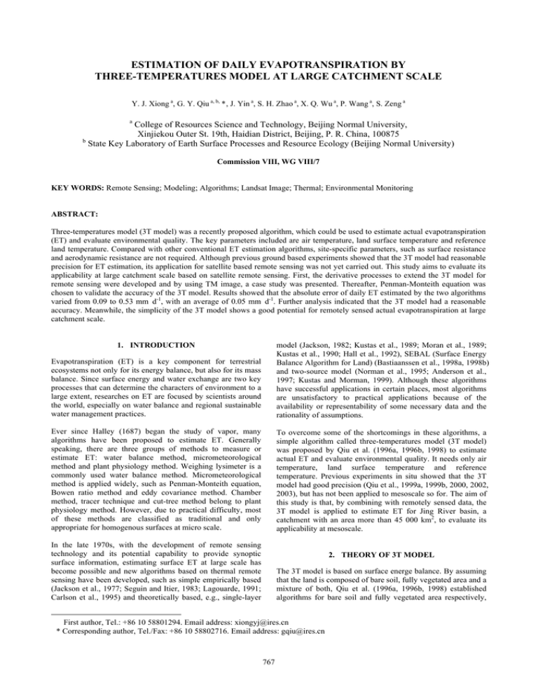
ESTIMATION OF DAILY EVAPOTRANSPIRATION BY
THREE-TEMPERATURES MODEL AT LARGE CATCHMENT SCALE
Y. J. Xiong a, G. Y. Qiu a, b, *, J. Yin a, S. H. Zhao a, X. Q. Wu a, P. Wang a, S. Zeng a
a
College of Resources Science and Technology, Beijing Normal University,
Xinjiekou Outer St. 19th, Haidian District, Beijing, P. R. China, 100875
b
State Key Laboratory of Earth Surface Processes and Resource Ecology (Beijing Normal University)
Commission VIII, WG VIII/7
KEY WORDS: Remote Sensing; Modeling; Algorithms; Landsat Image; Thermal; Environmental Monitoring
ABSTRACT:
Three-temperatures model (3T model) was a recently proposed algorithm, which could be used to estimate actual evapotranspiration
(ET) and evaluate environmental quality. The key parameters included are air temperature, land surface temperature and reference
land temperature. Compared with other conventional ET estimation algorithms, site-specific parameters, such as surface resistance
and aerodynamic resistance are not required. Although previous ground based experiments showed that the 3T model had reasonable
precision for ET estimation, its application for satellite based remote sensing was not yet carried out. This study aims to evaluate its
applicability at large catchment scale based on satellite remote sensing. First, the derivative processes to extend the 3T model for
remote sensing were developed and by using TM image, a case study was presented. Thereafter, Penman-Monteith equation was
chosen to validate the accuracy of the 3T model. Results showed that the absolute error of daily ET estimated by the two algorithms
varied from 0.09 to 0.53 mm d-1, with an average of 0.05 mm d-1. Further analysis indicated that the 3T model had a reasonable
accuracy. Meanwhile, the simplicity of the 3T model shows a good potential for remotely sensed actual evapotranspiration at large
catchment scale.
Evapotranspiration (ET) is a key component for terrestrial
ecosystems not only for its energy balance, but also for its mass
balance. Since surface energy and water exchange are two key
processes that can determine the characters of environment to a
large extent, researches on ET are focused by scientists around
the world, especially on water balance and regional sustainable
water management practices.
model (Jackson, 1982; Kustas et al., 1989; Moran et al., 1989;
Kustas et al., 1990; Hall et al., 1992), SEBAL (Surface Energy
Balance Algorithm for Land) (Bastiaanssen et al., 1998a, 1998b)
and two-source model (Norman et al., 1995; Anderson et al.,
1997; Kustas and Morman, 1999). Although these algorithms
have successful applications in certain places, most algorithms
are unsatisfactory to practical applications because of the
availability or representability of some necessary data and the
rationality of assumptions.
Ever since Halley (1687) began the study of vapor, many
algorithms have been proposed to estimate ET. Generally
speaking, there are three groups of methods to measure or
estimate ET: water balance method, micrometeorological
method and plant physiology method. Weighing lysimeter is a
commonly used water balance method. Micrometeorological
method is applied widely, such as Penman-Monteith equation,
Bowen ratio method and eddy covariance method. Chamber
method, tracer technique and cut-tree method belong to plant
physiology method. However, due to practical difficulty, most
of these methods are classified as traditional and only
appropriate for homogenous surfaces at micro scale.
To overcome some of the shortcomings in these algorithms, a
simple algorithm called three-temperatures model (3T model)
was proposed by Qiu et al. (1996a, 1996b, 1998) to estimate
actual ET and evaluate environmental quality. It needs only air
temperature, land surface temperature and reference
temperature. Previous experiments in situ showed that the 3T
model had good precision (Qiu et al., 1999a, 1999b, 2000, 2002,
2003), but has not been applied to mesoscale so for. The aim of
this study is that, by combining with remotely sensed data, the
3T model is applied to estimate ET for Jing River basin, a
catchment with an area more than 45 000 km2, to evaluate its
applicability at mesoscale.
1. INTRODUCTION
In the late 1970s, with the development of remote sensing
technology and its potential capability to provide synoptic
surface information, estimating surface ET at large scale has
become possible and new algorithms based on thermal remote
sensing have been developed, such as simple empirically based
(Jackson et al., 1977; Seguin and Itier, 1983; Lagouarde, 1991;
Carlson et al., 1995) and theoretically based, e.g., single-layer
2. THEORY OF 3T MODEL
The 3T model is based on surface energe balance. By assuming
that the land is composed of bare soil, fully vegetated area and a
mixture of both, Qiu et al. (1996a, 1996b, 1998) established
algorithms for bare soil and fully vegetated area respectively,
First author, Tel.: +86 10 58801294. Email address: xiongyj@ires.cn
* Corresponding author, Tel./Fax: +86 10 58802716. Email address: gqiu@ires.cn
767
The International Archives of the Photogrammetry, Remote Sensing and Spatial Information Sciences. Vol. XXXVII. Part B8. Beijing 2008
where Tcp and Rnp are, respectively, temperature and net
radiation of the imitation canopy (reference site).
thereafter fractional vegetation cover was introduced to
calculate ET for the mixture of both by weighing the soil
evaporation and vegetation transpiration.
Thus, when combining Eq. (1), Eq. (2) and Eq. (5), formula of
transpiration (T) for fully vegetated area can be obtained as
According to the general energy balance equation, energy
exchange just above the bare soil can be express as
LE = Rn -G - H
T −T
LT = Rn − Rn p c a
Tcp −Ta
(1)
where LE is the latent heat flux, of which L is the latent heat of
vaporization with a value of 2.49×106 W/(m2 mm) and E is the
soil evaporation; Rn is the net radiation at the soil surface in
W/m2; G is soil heat flux in W/m2; H is the sensible heat flux
between soil and atmosphere in W/m2, which can be derived
from the following equation as
where Tc is vegetation canopy temperature.
By introducing the fractional vegetation cover, f, ranging from
0 to 1 (0 for non-vegetation cover and 1 for fully vegetation
cover), ET for soil and vegetation mixed area can be weighed as
ET =(1− f ) E + fT
H=
ρ C p (Ts −Ta )
ra
(2)
f=
By introducing a dry soil without evaporation (reference surface,
E=0), Qiu et al. (1998) assumed that the atmosphere condition
around the reference surface might not be significantly changed
and the aerodynamic resistance of the dry soil and the around
drying soil was the same, under this condition ra of the drying
soil could be calculated by combining Eq. (1) and Eq. (2).
ρ C p (Tsd −Ta )
(7)
where f is defined by Kerr et al. (1992) as
where ρ is the air density in kg/m3, Cp is the specific heat at
constant pressure in MJ/(kg ℃); Ts is the soil surface
temperature and Ta is the air temperature in degree; ra is the
aerodynamic resistance in s/m, the diffusion resistance of the air
layer.
ra =
(6)
NDVI − NDVI min
NDVI max − NDVI min
(8)
where NDVI (normalized difference vegetation index) can be
retrieved from reflectance of red and near-infrared band, αr for
the former and αnir for the latter, of remotely sensed data using
the following equation:
α −α
NDVI = nir r
α nir +α r
(9)
(3)
where NDVImax and NDVImin, correspond to the values of NDVI
for bare soil and a surface with a fractional vegetation cover of
l00%, respectively.
where Tsd, Rnd and Gd are, respectively, soil temperature, net
radiation and soil heat flux of the dry soil (reference site).
The other two kind of unknown parameters in the 3T model are
net radiation Rn and soil heat flux G. If the model is used on
small scale, e.g., on plot, these two parameters can be measured;
if the scale becomes larger, especially to meoscale, it is difficult
to measure Rn or G. In this case, remote sensing could be an
effective alternative method, and Rn and G can be estimated
using the flowing algorithms:
Rnd −Gd
When combining Eqs. (1) to (3), evaporation (E) for bare soil
can be derived by
T −T
LE = Rn −G −( Rnd −Gd ) s a
Tsd −Ta
(4)
Rn = Rswd − Rswu + Rlwd − Rlwu
With the same method and by introducing an imitation canopy
(a canopy without transpiration, T=0), ra of the vegetation could
be estimated using the following formula:
ra =
ρ C p (Tcp −Ta )
Rnp
(10)
where Rswd, Rswu, Rlwd and Rlwu stand for the incoming shortwave
and outgoing shortwave radiation and incoming longwave and
outgoing longwave radiation respectively.
(5)
768
Rswd =τ ⋅S ⋅E0 ⋅cos θ
(11)
τ =0.75+ 2×10−5×h
(12)
The International Archives of the Photogrammetry, Remote Sensing and Spatial Information Sciences. Vol. XXXVII. Part B8. Beijing 2008
E0 =1+ 0.033cos(2π d n / 365)
(13)
ETd =
where τ is the atmospheric transmittance coefficient and can be
derived from measurements at the meteorological station, or
from elevation (h, in meter) using Eq. (12) proposed by Allen et
al. (1994); S is the solar constant (1 367 W/m2); E0 is the
eccentricity correction factor and can be calculated with dn
(Allen et al., 1998), the number of the day in the year between 1
(1 January) and 365 or 366 (31 December); θ is the solar zenith
angle in radian.
Rswu =α Rswd
ε a =9.2×10−6 ×(Ta + 273.15)2
(14)
input parameter
source
advantages
air
meteorological
temperature station
easy to obtain
surface retrieve from remote
temperature sensing data
there are land surface
temperature products, or
the algorithms to retrieve
land surface temperature
are mature
net radiation
retrieve from remote
sensing data
the algorithms to retrieve
net radiation are mature
soil heat
flux
calculate from net
radiation
easy to calculate
(15)
(16)
where σ is the Stefan-Boiltzmann constant (5.67×10-8 W/(m2
K4)); εa is the atmospheric emissivity and can be calculated
from practical approaches such as Eq. (16) proposed by
Swinbank (Campbell and Norman,1998); Ta is air temperature
in Celsius.
Rlwu =σ ⋅ε s ⋅Ts 4
(19)
where ETd is daily ET and ETi is instantaneous one at any timeof-day; NE is the daily ET hours and equals to the time interval
between sunrise and sunset minus two; t is the time interval
between sunrise and the data-collecting time of the satellite
sensor passing by.
where α is the surface albedo, and can be calculated with
remote sensing data as proposed by Liang (2001).
Rlwd =σ ⋅ε a ⋅(Ta + 273.15)4
ETi ⋅ 2 N E
π ⋅ sin(π ⋅ t / N E )
the parameters of
parameters reference site can be
of reference obtained from the
site
above
results
correspondingly
reference
site
is
determined
by
the
maximum
surface
temperature, thus it is
easy to obtain
Table 1 Parameters needed in the 3T model
(17)
3. MODEL APPLICATION
where εs is surface emissivity and Ts is land surface temperature
in Kelvin, which can be retrieved from remote sensing data.
In this study, one TM data inside Jing River basin, China
(Figure 1), scanned in August 28th, 1987 from path 128 and row
35, was adopted as the original data to retrieve land surface
temperature (LST), using the mono-window algorithm proposed
by Qin et al. (2001). However, it was difficult to separate soil
temperature from vegetation canopy temperature with the
adopted algorithm, hence the retrieved LST was assumed to be
the temperature of bare soil (Ts) where NDVI less than 0.05, or
of canopy (Tc) where NDVI larger than 0.70, and when DNVI
ranging between 0.05 and 0.70, the retrieved LST was assumed
to be the mixture of soil and canopy, which could be departed
through Eq. (20) (Lhomme et al., 1994).
Soil heat flux can be estimated from net radiation as suggested
by Su et al. (2001)
G = Rn ⋅[ Γc + (1− f )⋅( Γ s −Γc )]
(18)
where Гc and Гs are empirical coefficient: Гs = 0.315 (Kustas
and Daughtry, 1990) and Гc = 0.05 (Monteith, 1973).
When applying the 3T model at large catchment scale, it is
important to find out the reference site of bare soil or fully
vegetated area. Usually the temperature of the reference site has
the maximum value, according to this, the reference site can be
determined. Thus reference temperature of bare soil or canopy,
Tsd or Tcp, is respectively obtained as the maximum temperature
of bare soil or canopy, Ts or Tc, in a given image or in a given
area, with which reference value of Rn or G can be calculated.
f ⋅ Tcm + (1 − f ) ⋅ Tsm = Tmix
Tsm − Tcm = a ⋅ (Tmix − Ta ) m
(20)
where Tcm and Tsm are, respectively, the temperature of the
foliage and the soil surface; Tmix is the radiometric surface
temperature, which was assumed to be the retrieved LST; a and
m are empirical coefficients, because approaches to adjust these
parameters are not currently available so that the values of a =
0.1 and m = 2 given by Lhomme et al. (1994) were used.
With all the needed inputs of 3T model (Table 1) are available,
instantaneous ET can be estimated; thereafter daily ET can be
derived by (Xie et al., 1991)
769
The International Archives of the Photogrammetry, Remote Sensing and Spatial Information Sciences. Vol. XXXVII. Part B8. Beijing 2008
The air temperature was interpolated with daily values from
several national meteorological stations (Figure 1). Based on
the results of LST, interpolated air temperature and some
auxiliary data such as DEM, net radiation and soil heat flux
were calculated with algorithms in section 2.
By using the 3T model, the instantaneous ET was estimated: the
maximum value was 1.5 mm/h; the minimum value was 0 mm/h;
and the average was 0.46 mm/h, as shown in Figures 2 and 3,
based on which daily ET could be calculated (Figure 4).
Figure 3 Histogram of the estimated instantaneous ET (mm/h)
Figure 1 Location of the study area
Figure 4 Daily ET (mm/d) based on TM image on August 28th,
1987 in Jing River basin
4. MODEL VALIDATION AND DISCUSSION
In order to validate the accuracy of the 3T model, its results
were compared with the results of another study in Jing River
basin, in which the ET was estimated using Penman-Monteith
(P-M) equation by SWAT model (Kannan et al., 2007). One
defect was that the ET resulted from SWAT model was not
pixel based, instead it divided the whole river basin into a
couple of sub-basins and each sub-basin gave one ET value.
Therefore, the validation was based on sub-basin, and daily ET
of each sub-basin estimated from the 3T model was averaged
for the comparison.
Figure 2 Instantaneous ET (mm/h) estimated by the 3T model
based on TM image on August 28th, 1987
As the area of Jing River basin was larger than one TM image,
eight intact sub-basins inside the TM boundary were chosen for
a meaningful validation (Figure 4), but TM data was covered by
770
The International Archives of the Photogrammetry, Remote Sensing and Spatial Information Sciences. Vol. XXXVII. Part B8. Beijing 2008
cloud in the number six sub-basin and the comparison of this
region was eliminated (Table 2). In the seven regions, the
maximum daily ET estimated by Penman-Monteith equation
was 2.88 mm/d, whereas 3.74 mm/d for the 3T model, and the
minimum value estimated by Penman-Monteith equation was
0.92 mm/d, while 2.35 mm/d for the 3T model. In the whole,
the maximum absolute error was 2.81 mm/d whereas the
minimum was 0.09 mm/d and 0.63 mm/d in average. The
RMSE (Root Mean Square Error) was 2.92 mm/d for these
seven basins. The results of the other eight partial sub-basin
extended outside the TM boundary were also given in Table 2,
and the absolute error varied differently.
vegetated areas, with 5.41 mm/d on average, and ET from the
mixed land was in the middle, with 2.81 mm/d on average.
5. CONCLUSION
This study provided a process to extent the 3T model for
estimating the ET of larger catchment by remote sensing. After
comparing with P-M equation, it was concluded that the 3T
model had a reasonable accuracy. Meanwhile, the simplicity of
the 3T model shows a good potential for remotely sensed actual
evapotranspiration at large catchment scale.
However, some ET values estimated by SWAT model might be
unreasonable as their showed abnormal value. For instance, the
value of sub-basin 12 was only 0.92 mm/d, but in this region, at
least one third area was covered by forest, how could the
transpiration have such a low value? In addition, if considering
the average value of the two methods, it was found that the
absolute error was only 0.05 mm/d for the six intact sub-basins
whereas 0.02 mm/d for the whole sub-basins list in Table 2.
ET (mm/d)
No. of
sub-basin
intacta
SWAT (P-M)
3T
6
1.88
*
*
7
2.35
2.44
0.10
9
2.40
2.49
0.09
11
2.56
2.88
0.32
12
0.92
3.74
2.81
15
2.39
2.51
0.12
16
2.88
2.35
0.53
19
2.84
2.44
0.40
average
2.47
2.52
0.05
3
2.86
2.34
0.52
4
3.35
2.73
0.62
5
0.92
3.04
2.12
8
3.37
2.42
0.96
10
3.42
2.41
1.01
13
3.68
2.39
1.29
14
2.87
2.50
0.37
17
3.44
2.11
1.33
23
2.93
3.27
0.34
25
2.94
3.63
0.69
b
Partiala
Absolute error
(mm/d)
Figure 5 Statistical results of daily ET estimated by the 3T
model for different covers on August 28th, 1987
REFERENCES
Allen, R.G., Smith, M., Pereira, L.S., Perrier, A., 1994. An
Update for the Calculation of Reference Evapotranspiration.
ICID Bulletin, 43 (2), pp. 35-92.
Notice:
a: intact means the boundary of each sub-basin was in the adopted TM
imagery, whereas partial means a little part of each sub-basin was
outside of the imagery; half of No. 6 watershed is covered by cloud in
the TM imagery and the estimated value was eliminated.
b: the average value did not include the value of sub-basin 12.
Anderson, M. C., Norman, J. M., Diak, G. R., Kustas, W. P.,
Mecikalski, J. R., 1997. A two-source time-integrated model for
estimating surface fluxes using thermal infrared remote sensing.
Remote Sensing of Environment, 60 (2), pp. 195-216.
Table 2 Comparing of the estimated daily ET between the 3T
model and the P-M equation (SWAT)
Bastiaanssen, W. G. M., Menenti, M., Feddes, R. A., Holtslag,
A. A. M., 1998a. A remote sensing surface energy balance
algorithm for land (SEBAL). 1. Formulation. Journal of
Hydrology, 212–213, pp. 198–212.
Statistical results further showed the reasonability of the 3T
model (Figure 5). The minimum ET was from bare soil, with
2.25 mm/d on average, the maximum ET was from fully
771
The International Archives of the Photogrammetry, Remote Sensing and Spatial Information Sciences. Vol. XXXVII. Part B8. Beijing 2008
Bastiaanssen, W. G. M., Pelgrum, H., Wang, J., Ma, Y.,
Moreno, J. F., Roerink, G. J., 1998b. A remote sensing surface
energy balance algorithm for land (SEBAL). Part 2, pp.
Validation. Journal of Hydrology, 212–213, pp. 213–229.
Lhomme, J. –P., Monteny, B., Amadou, M., 1994. Estimating
sensible heat flux from radiometric temperature over sparse
millet. Agricultural and Forest Meteorology, 68, pp. 77-91.
Liang, S. L., 2001. Narrowband to broadband conversions of
land surface albedo I Algorithms. Remote Sensing of
Environment, 76 (2), pp. 213-238.
Campbell, G. S., Norman, J. M., 1998. An introduction to
environmental biophysics (Second edition). New York, Springer
Press, pp. 164.
Monteith, J. L., 1973. Principles of environmental physics
(Second edition). London, Edward Arnold Press, pp. 241.
Carlson, T. N., Capehart, W. J., Gillies, R. R., 1995. A new
look at the simplified method for remote sensing of daily
evapotranspiration. Remote Sensing of Environment, 54, pp.
161-167.
Moran, M. S., Jackson, R. D., Raymond, L. H., Gay, L. W.,
Slater, P. N., 1989. Mapping surface energy balance
components by combining landsat thematic mapper and groundbased meteorological data. Remote Sensing of Environment,
30(1), pp. 77-87.
Hall, F. G., Huemmrich, K. F., Goetz, S. J., Sellers, P. J.,
Nickerson, J. E., 1992. Satellite remote sensing of surface
energy balance: success, failures and unresolved issues in FIFE.
Journal of Geophysics Research, 97, pp. 19061-19089.
Norman, J. M., Kustas, W. P., Humes, K. S., 1995. Source
approach for estimating soil and vegetation energy fluxes in
observations of directional radiometric surface temperature.
Agricultural and Forest Meteorology, 77 (3-4), pp. 263-293.
Hally, E., 1687. An estimate of the quantity of vapor raised out
of the sea by warmth of sun. Philosophical Transactions of the
Royal Society of London, 16, pp. 366-370.
Qin, Z., Karnieli, A., Berliner, P., 2001. A mono-window
algorithm for retrieving land surface temperature from Landsat
TM data and its application to the Israel-Egypt border region.
International Journal of Remote Sensing, 2 (18), pp. 3719-3746.
Jackson, R. D., 1982. Soil moisture inferences from thermalinfrared measurements of vegetation temperatures. IEEE
Transition Geosciences of Remote Sensing, 20, pp. 282-285.
Jackson, R. D., Reginato, R. J., Idso, S. B., 1977. Wheat canopy
temperature: a practical tool for evaluating water requirements,
Water Resource Research, 13, pp. 651-656.
Qiu, G. Y., Yano, T., Momii, K., 1996a. Estimation of plant
transpiration by imitation leaf temperature.Ⅰ. Theoretical
consideration and field verification. Transactions of the
Japanese society of irrigation, Drainage and Reclamation
Engineering, 64, pp. 401-410.
Kannan, N., White, S. M., Worrall, F., Whelan, M. J., 2007.
Sensitivity analysis and identification of the best
evapotranspiration and runoff options for hydrological
modelling in SWAT-2000. Journal of Hydrology, 332 (3-4), pp.
456-466.
Qiu, G. Y., Yano, T., Momii, K., 1996b. Estimation of plant
transpiration by imitation leaf temperature.Ⅱ. Application of
imitation leaf temperature for detection of crop water stress.
Transactions of the Japanese society of irrigation, Drainage
and Reclamation Engineering, 64, pp. 767-773.
Kerr, Y. H., Lagouarde, J. P., Imbernon, J., 1992. Accurate land
surface temperature retrieval from AVHRR data with use of an
improved split window algorithm. Remote Sensing of
Environment, 41 (2-3), pp. 197-209.
Qiu, G. Y., Yano, T., Momii, K., 1998. An improved
methodology to measure evaporation from bare soil based on
comparison of surface temperature with a dry soil. Journal of
Hydrology, 210 (1-4), pp. 93-105.
Kustas, W. P., Choudhury, B. J., Moran, M. S., Reginato, R. J.,
Jackson, R. D., Gay, L. W., Weaver, H. L., 1989.
Determination of sensible heat flux over sparse canopy using
thermal infrared data. Agricultural and Forest Meteorology, 44
(3-4), pp. 197-216.
Qiu, G. Y., Ben-Asher, J., Yano, T., Momii, K., 1999a.
Estimation of soil evaporation using the differential temperature
method. Soil Science Society of American Journal, 63, pp.
1608-1614.
Kustas, W. P., Daughtry, C. S. T., 1990. Estimation of the soil
heat flux/net radiation ratio from spectral data. Agricultural and
Forest Meteorology, 49 (3), pp. 205-223.
Qiu, G. Y., Momii, K., Yano, T., Lascano, R. J., 1999b.
Experimental verification of a mechanistic model to partition
evapotranspiration into soil water and plant evaporation.
Agricultural and Forest Meteorology, 93 (2), pp. 79-93.
Kustas, W. P., Moran, M. S., Jackson, R. D., Gay, L. W., Duell,
L. F. W., Kunkel, K. E., Matthias, A. D., 1990. Instantaneous
and daily values of the surface energy balance over agricultural
fields using remote sensing and a reference field in an arid
environment. Remote Sensing of Environment, 32 (2-3), pp.
125-141.
Qiu, G. Y., Miyamoto, K., Sase, S., Okushima, L., 2000.
Detection of crop transpiration and water stress by temperature
related approach under the field and greenhouse conditions.
JARQ-Japan Agricultural Research Quarterly, 34, pp. 29-37.
Kustas, W. P., Norman, J.M., 1999. Evaluation of soil and
vegetation heat flux predictions using a simple two-source
model with radiometric temperatures for partial canopy cover.
Agricultural and Forest Meteorology, 94 (1), pp. 13–29.
Qiu, G. Y., Miyamoto, K., Sase, S., Gao, Y., Shi, P. J., Yano, T.,
2002. Comparison of the three temperatures and conventional
models for estimation of transpiration. JARQ-Japan
Agricultural Research Quarterly, 36 (2), pp. 73-82.
Lagouarde, J. P., 1991. Use of NOAA-AVHRR data combined
with an agrometeorological model for evaporation mapping.
International Journal of Remote Sensing, 12 (9), pp. 1853-1864.
Qiu, G. Y., Sase, S., Shi, P. J., Ding, G. D., 2003. Theoretical
analysis and experimental verification of a remotely measurable
772
The International Archives of the Photogrammetry, Remote Sensing and Spatial Information Sciences. Vol. XXXVII. Part B8. Beijing 2008
plant transpiration coefficient. JARQ-Japan
Research Quarterly, 37 (3), pp. 141-149.
Agricultural
Remote Sensing of Environment China, 6 (4), pp. 253-259 (in
Chinese).
Seguin, B., Itier, B., 1983. Using midday surface temperature to
estimate daily evaporation from satellite thermal IR data.
International Journal of Remote Sensing, 4, pp. 473-383.
ACKNOWLEDGEMENTS
This research was funded by National Natural Science
Foundation of China (40771037) and National Basic Research
Program of China (2006CB400505).
Su, Z., Schmugge, T., Kustas, W. P., Massman, W. J., 2001. An
evaluation of two models for estimation of the roughness height
for heat transfer between the land surface and the atmosphere.
Journal of Applied Meteorology, 40 (11), pp. 1922-1951.
Xie, X. Q., 1991. Estimation of daily evapo-transpiration (ET)
from one time-of-day remotely sensed canopy temperature.
773
The International Archives of the Photogrammetry, Remote Sensing and Spatial Information Sciences. Vol. XXXVII. Part B8. Beijing 2008
774