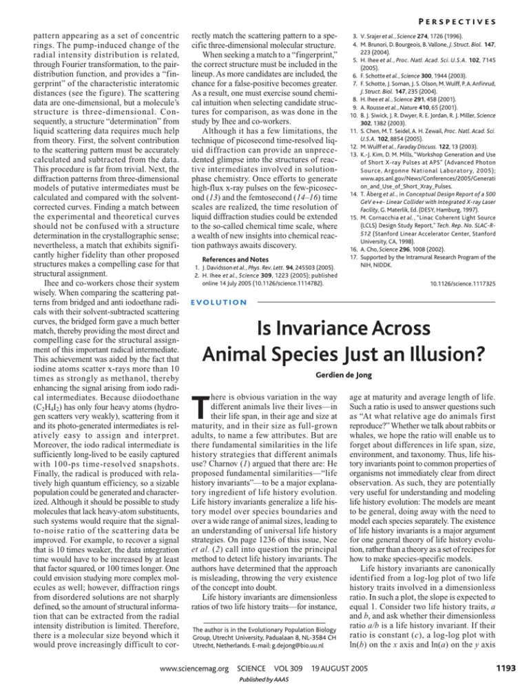
PERSPECTIVES
pattern appearing as a set of concentric
rings. The pump-induced change of the
radial intensity distribution is related,
through Fourier transformation, to the pairdistribution function, and provides a “fingerprint” of the characteristic interatomic
distances (see the figure). The scattering
data are one-dimensional, but a molecule’s
structure is three-dimensional. Consequently, a structure “determination” from
liquid scattering data requires much help
from theory. First, the solvent contribution
to the scattering pattern must be accurately
calculated and subtracted from the data.
This procedure is far from trivial. Next, the
diffraction patterns from three-dimensional
models of putative intermediates must be
calculated and compared with the solventcorrected curves. Finding a match between
the experimental and theoretical curves
should not be confused with a structure
determination in the crystallographic sense;
nevertheless, a match that exhibits significantly higher fidelity than other proposed
structures makes a compelling case for that
structural assignment.
Ihee and co-workers chose their system
wisely. When comparing the scattering patterns from bridged and anti iodoethane radicals with their solvent-subtracted scattering
curves, the bridged form gave a much better
match, thereby providing the most direct and
compelling case for the structural assignment of this important radical intermediate.
This achievement was aided by the fact that
iodine atoms scatter x-rays more than 10
times as strongly as methanol, thereby
enhancing the signal arising from iodo radical intermediates. Because diiodoethane
(C2H4I2) has only four heavy atoms (hydrogen scatters very weakly), scattering from it
and its photo-generated intermediates is relatively easy to assign and interpret.
Moreover, the iodo radical intermediate is
sufficiently long-lived to be easily captured
with 100-ps time-resolved snapshots.
Finally, the radical is produced with relatively high quantum efficiency, so a sizable
population could be generated and characterized. Although it should be possible to study
molecules that lack heavy-atom substituents,
such systems would require that the signalto-noise ratio of the scattering data be
improved. For example, to recover a signal
that is 10 times weaker, the data integration
time would have to be increased by at least
that factor squared, or 100 times longer. One
could envision studying more complex molecules as well; however, diffraction rings
from disordered solutions are not sharply
defined, so the amount of structural information that can be extracted from the radial
intensity distribution is limited. Therefore,
there is a molecular size beyond which it
would prove increasingly difficult to cor-
rectly match the scattering pattern to a specific three-dimensional molecular structure.
When seeking a match to a “fingerprint,”
the correct structure must be included in the
lineup. As more candidates are included, the
chance for a false-positive becomes greater.
As a result, one must exercise sound chemical intuition when selecting candidate structures for comparison, as was done in the
study by Ihee and co-workers.
Although it has a few limitations, the
technique of picosecond time-resolved liquid diffraction can provide an unprecedented glimpse into the structures of reactive intermediates involved in solutionphase chemistry. Once efforts to generate
high-flux x-ray pulses on the few-picosecond (13) and the femtosecond (14–16) time
scales are realized, the time resolution of
liquid diffraction studies could be extended
to the so-called chemical time scale, where
a wealth of new insights into chemical reaction pathways awaits discovery.
References and Notes
1. J. Davidsson et al., Phys. Rev. Lett. 94, 245503 (2005).
2. H. Ihee et al., Science 309, 1223 (2005); published
online 14 July 2005 (10.1126/science.1114782).
3. V. Srajer et al., Science 274, 1726 (1996).
4. M. Brunori, D. Bourgeois, B. Vallone, J. Struct. Biol. 147,
223 (2004).
5. H. Ihee et al., Proc. Natl. Acad. Sci. U.S.A. 102, 7145
(2005).
6. F. Schotte et al., Science 300, 1944 (2003).
7. F. Schotte, J. Soman, J. S. Olson, M.Wulff, P. A. Anfinrud,
J. Struct. Biol. 147, 235 (2004).
8. H. Ihee et al., Science 291, 458 (2001).
9. A. Rousse et al., Nature 410, 65 (2001).
10. B. J. Siwick, J. R. Dwyer, R. E. Jordan, R. J. Miller, Science
302, 1382 (2003).
11. S. Chen, M. T. Seidel, A. H. Zewail, Proc. Natl. Acad. Sci.
U.S.A. 102, 8854 (2005).
12. M. Wulff et al., Faraday Discuss. 122, 13 (2003).
13. K.-J. Kim, D. M. Mills, “Workshop Generation and Use
of Short X-ray Pulses at APS” (Advanced Photon
Source, Argonne National Laboratory, 2005);
www.aps.anl.gov/News/Conferences/2005/Generati
on_and_Use_of_Short_Xray_Pulses.
14. T. Åberg et al., in Conceptual Design Report of a 500
GeV e+e- Linear Collider with Integrated X-ray Laser
Facility, G. Materlik, Ed. (DESY, Hamburg, 1997).
15. M. Cornacchia et al., “Linac Coherent Light Source
(LCLS) Design Study Report,” Tech. Rep. No. SLAC-R512 (Stanford Linear Accelerator Center, Stanford
University, CA, 1998).
16. A. Cho, Science 296, 1008 (2002).
17. Supported by the Intramural Research Program of the
NIH, NIDDK.
10.1126/science.1117325
E VO L U T I O N
Is Invariance Across
Animal Species Just an Illusion?
Gerdien de Jong
here is obvious variation in the way
different animals live their lives—in
their life span, in their age and size at
maturity, and in their size as full-grown
adults, to name a few attributes. But are
there fundamental similarities in the life
history strategies that different animals
use? Charnov (1) argued that there are: He
proposed fundamental similarities—“life
history invariants”—to be a major explanatory ingredient of life history evolution.
Life history invariants generalize a life history model over species boundaries and
over a wide range of animal sizes, leading to
an understanding of universal life history
strategies. On page 1236 of this issue, Nee
et al. (2) call into question the principal
method to detect life history invariants. The
authors have determined that the approach
is misleading, throwing the very existence
of the concept into doubt.
Life history invariants are dimensionless
ratios of two life history traits—for instance,
T
The author is in the Evolutionary Population Biology
Group, Utrecht University, Padualaan 8, NL-3584 CH
Utrecht, Netherlands. E-mail: g.dejong@bio.uu.nl
www.sciencemag.org
SCIENCE
VOL 309
Published by AAAS
age at maturity and average length of life.
Such a ratio is used to answer questions such
as “At what relative age do animals first
reproduce?” Whether we talk about rabbits or
whales, we hope the ratio will enable us to
forget about differences in life span, size,
environment, and taxonomy. Thus, life history invariants point to common properties of
organisms not immediately clear from direct
observation. As such, they are potentially
very useful for understanding and modeling
life history evolution: The models are meant
to be general, doing away with the need to
model each species separately. The existence
of life history invariants is a major argument
for one general theory of life history evolution, rather than a theory as a set of recipes for
how to make species-specific models.
Life history invariants are canonically
identified from a log-log plot of two life
history traits involved in a dimensionless
ratio. In such a plot, the slope is expected to
equal 1. Consider two life history traits, a
and b, and ask whether their dimensionless
ratio a/b is a life history invariant. If their
ratio is constant (c), a log-log plot with
ln(b) on the x axis and ln(a) on the y axis
19 AUGUST 2005
1193
PERSPECTIVES
15
5
Slope = 1
0
–4
0
8
4
12
16
–5
–10
ln(adult body size)
What log-log plots reveal about life histories.
The log-log plot shows a life history invariant.
Size at maturity seems a constant fraction of
adult size for all animals over a body size range
from 6 × 10–2 to 6 × 105. The slope equals 1.01
and R2 equals 0.95.The life history invariant estimated would equal 0.34. The plot has been generated from values that were randomly produced according to Nee et al. (2), indicating the
misleading nature of regression analysis.
invariant: a slope of 1 and an R2 of >0.95.
More null models followed (5, 6), using different random distributions of traits. But
Nee et al. (2) describe the general rationale
of how slopes of 1 at high R2 arise in log-log
plots, independent of the distributions of the
traits. The culprit is a variable on the y axis
that is a fraction of the x-variable: The plot
is of y = cx, with c < 1. In a log-log plot of cx
versus x, a slope of 1 follows automatically.
A wide range on the x axis—from rabbit to
whale—guarantees a high R2. The evidence
for life history invariants vanishes as the
method of finding them evaporates.
Suppose full-grown body size is plotted
on the x axis, and size at maturity of the
same individual on the y axis [see the bottom figure; (4)]. Size at maturity might be
any fraction of full-grown body size, with
10,000
fractions c = 0.1, 0.2, …, 0.9 in nine different groups of animals. Each animal group
has its own relative size at maturity. Relative
size at maturity is invariant within each
group but varies among groups. All possible
combinations of full-grown body size and
size at maturity can be found over the nine
groups. When data from multiple animal
groups are plotted directly, the variance
among them is quite apparent. The same
data can be depicted in a log-log plot for the
total range of body sizes, still distinguishing
each animal group. Each group now has its
own line ln(y) = ln(c) + ln(x), all with a
slope of 1 but each with different intercepts
ln(c), again revealing variation between animal groups. However, if the same data are
again depicted on a log-log plot, but without
differentiation as to which animal group the
data points belong, a single regression line
can be drawn over all groups together that
now seems to indicate a life history invariant ratio of body size at maturity to fullgrown body size over all groups. The
regression analysis is therefore misleading.
If life history invariants are important in
evolution, we expect them to surface in
models that use their component variables.
That would validate the idea of invariants,
especially if a model restricts them to certain values. Kozlowski (7) modeled growth
in animals and optimal body size. In his
model and simulation, many life history
variables that partake in life history invariants can be evaluated. The slopes in log-log
plots of model values are 1 for the proposed
life history invariants. Yet very much variation in the simulated traits and their ratios
exists, and direct observation of the values
will not give the impression of life history
invariants. Kozlowski (7) concluded that
“Charnov’s life history invariants can be
10
Relative size at maturity differs
among nine groups
of animals
8000
Size at maturity
Regression analysis
indicates a life
history
invariant
10
ln(size at maturity)
would show points on a line def ined by
ln(a) = ln(c) + ln(b), with a slope of 1 and
intercept ln(c) (see the top figure). The line
is the regression line and the intercept can
be used to estimate the life history invariant, c. A log-log plot of two traits involved
in a life history invariant leads to a slope of
1 with all variation in the dependent variable on the y axis explained by the variable
on the x axis (that is, R 2 = 1 for an ideal
invariant where R2 of the regression is the
proportion of the variation in the dependent
variable a explained by the variation in the
independent variable b). An empirically
determined slope of 1 at high explained
variance R 2 has therefore been taken to
indicate a life history invariant. This is
common experimental logic, but treacherous, as it disregards the potential existence
of other ways to arrive at the predicted
slope of 1 and very high R2. If a life history
invariant is the only way to arrive at a slope
of 1 and very high R2, then one can conclude from an empirical slope of 1 and very
high R2 that a life history invariant exists.
Many such log-log plots of traits that
indicate potential life history invariants
exist. Allsop and West (3) presented data on
relative body size at sex change for animals
ranging from a 2-mm shrimp to a 1.5-m
fish. The log-log plot of body size at sex
change versus maximum body size showed
a slope of 1.05, and all the points were near
the regression line, with R2 = 0.98. The life
invariant “relative body size at sex change”
was perfectly present.
Buston et al. (4) then threw a spanner in
the works. Commenting on Allsop and
West’s data, Buston et al. pointed out that
random distributions of both total body size
and size at sex change lead to identical
properties in a log-log plot as a life history
Log-log plot of the same data
shows relative size varies
across groups
8
6000
6
4000
4
2000
2
0
8
All slopes = 1
6
2000
4000
6000
8000
10,000
Slope = 1
4
2
0
0
Log-log plot of the same data
with regression analysis
now indicates a life
history invariant
10
0
2
4
6
8
10
0
0
2
4
6
8
10
Adult body size
A mirage of invariance. Consider nine groups of animals that differ in whether
they mature at large or small size. In group 1, size at maturity equals one-tenth
of adult body size; in group 2, size at maturity equals two-tenths of adult body
size, and so on. [Adapted from (4)] (Left) Size at maturity is plotted as a function of body size for the nine groups and for seven body sizes: 10, 10√10, 100,
100√10, 1000, 1000√10, and 10,000. The lines give y = cx for nine values of c
(c = 0.1, 0.2, …, 0.9). (Middle) The same data are plotted on a log-log plot. The
1194
19 AUGUST 2005
VOL 309
lines are now ln(y) = ln(c) + ln(x), and all lines show a slope of 1 but possess different intercepts. Within each group, the relative size at maturity is invariant,
but not across groups. (Right) A log-log plot of the same data but without
assignment to different animal groups reveals a regression line with a slope of
1, an intercept of –0.88, a high R2 of 0.92, and a life history invariant of 0.42.The
estimated “life history invariant” is actually a complicated way of averaging all
nine values for c. Any conclusion that a life history invariant exists is spurious.
SCIENCE
Published by AAAS
www.sciencemag.org
PERSPECTIVES
called invariants only in the sense that the
regression lines between their components
have slopes close to +1 or –1.”
Life history evolution is not the only
field where invariants or universal constants
are proposed. The Universal Temperature
Dependence of metabolism proposal asserts
that the metabolism of all organisms can be
described by a single equation (8). Scaling
laws (as, for instance, basic metabolic rate
scale as mass to the power 3/4 ) are called
universal over all life (9, 10). This hankering
for universal explanations has been criticized not only on technical grounds (11) but
also for ignoring biology and the variation
between organisms (12). Interesting biology
might not be in life history invariants but in
biological variation.
Consider again the issue of relative body
size at sex change. Allsop and West (3) collected data on this question and interpreted
their log-log plot as showing a life history
invariant indicating that a fundamental similarity exists among all animals in the fitness components leading to sex change.
However, looking at specific cases of sex
change does not strengthen that impression.
In both the clown fish and the bluebanded
goby, an individual’s sex is determined by
its rank in the social hierarchy. Among
clown fish, the largest fish of the group is
female, the second largest fish is male, and
lower ranking group members are queuing
for their turn to reproduce (13). Among
bluebanded gobies, the fish at the top of the
hierarchy is male and below him are several
breeding females; the group has no nonbreeding adults (14). In both fish species,
the second ranking member in the hierarchy
changes sex and starts growing in size when
the top brass exits (13, 14). The interesting
biology is to identify what determines differences such as those between these two
fish species.
This brings us back to species-specific
life histories and back to looking at biological mechanisms. If a fundamental similarity
does exist among all animals in the fitness
components leading to sex change, it has to
be shown that relative body size at sex
change for both the clown fish and the bluebanded goby can be directly described by
similar fitness relations. The model of optimal relative body size at sex change (15)
must be shown to work by direct estimation
of its parameters for both fish species, not
by log-log plot.
We should be wary of treating an average across species as an explanatory general life history invariant. That’s not to say
that we might not keep searching for
invariants that indicate fundamental similarities in the biology of all living organisms. We just need to know for certain how
to identify them.
References
1. E. L. Charnov, Life History Invariants: Some Explorations
of Symmetry in Evolutionary Ecology (Oxford Univ.
Press, Oxford, 1993).
2. S. Nee, N. Colegrave, S. A.West, A. Grafen, Science 309,
1236 (2005).
3. D. J. Allsop, S. A. West, Nature 425, 783 (2003).
4. P. M. Buston, P. L. Munday, R. R. Warner, Nature 428,
10.1038/nature02512 (2004).
5. A. Gardner, D. J. Allsop, E. L. Charnov, S. A. West, Am.
Nat. 165, 551 (2005).
6. R. Cipriani, R. Collin, J. Evol. Biol., 10.1111/j.
1420-09101.2005.00949.x (2005).
7. J. Kozlowski, Proc.R.Soc.London Ser.B 263, 559 (1996).
8. J. F. Gillooly, J. H. Brown, G. B. West, V. M. Savage, E. L.
Charnov, Science 293, 2248 (2001).
9. G. B. West, W. H. Woodruff, J. H. Brown, Proc. Natl.
Acad. Sci. U.S.A. 99, 2473 (2002).
10. G. B. West, J. H. Brown, Phys. Today 57, 36 (September
2004).
11. J. Kozlowski, M. Konarzewski, Funct. Ecol. 18, 283
(2004).
12. A. Clarke, Funct. Ecol. 18, 252 (2004).
13. P. Buston, Nature 424, 145 (2003).
14. E.W. Rodgers, S. Drane, M. S. Grober, Biol. Bull. 208, 120
(2005).
15. E. L. Charnov, U. Skuladottir, Evol. Ecol. Res. 2, 1067
(2000).
10.1126/science.1117591
C H E M I S T RY
def initive experimental and theoretical
studies of reaction dynamics. On page
1227 of this issue, Juanes-Marcos et al. (6)
provide a novel topological argument to
show when the geometric phase is likely to
be observable in this hydrogen exchange
reaction and also clarify the findings of
David C. Clary
previous calculations.
To understand chemical reactions, theouantum mechanical effects such as chemical reactions are less certain. Studies rists solve the Schrödinger equation for the
tunneling through a classically of this effect have largely been directed at electrons to calculate potential energy surimpenetrable potential energy bar- the simplest chemical reaction, H + H2 → faces on which the nuclei move. These surrier have long been known to occur in H2 + H, which serves as the benchmark for faces are then used in quantum dynamical
chemical reactions (1). More subtle quancomputations that solve the Schrödinger
tum effects can also arise for reactions in
equation for the nuclei taking part in the
which two different electronic states touch
reaction at different energies (7). The nuclear
(that is, coincide in energy) to produce a
wave functions are calculated for different
Excited state
conical intersection (see the figure). An
values of the total angular momentum J of
example is the geometric or Berry phase,
the system of three hydrogen atoms, and
Energy
which refers to a change in sign of an electhese partial wave functions are
H + H2
tronic wave function when nuclei of atoms
summed to produce quantities
reactants
involved in the reaction complete an odd
that can be observed in molecunumber of loops around the conical interlar beam experiments such as
section (2–4). The effect of the geometric
the angular distributions of the
H2 + H
H2 + H
product
phase on the energy levels of bound-state
H2 + H products. These quanproduct
molecules is well understood (5).
tum dynamical calculations can
Ground state
However, the conditions under which the
be done with time-independent
geometric phase effect can be detected for
or time-dependent theory. One
Chemical topology. Conical intersection shown in plot of set of time-independent quanenergy versus two reaction coordinate dimensions with direct tum dynamical calculations on
The author is in the Department of Physical and
(red) and looping (blue) reaction paths.The cones correspond to an accurate potential energy
Theoretical Chemistry, University of Oxford, South
the upper excited-state and lower ground-state potential surface suggested that the geoParks Road, Oxford OX1 3QZ, UK. E-mail:
metric phase effect might be
david.clary@chem.ox.ac.uk
energy surfaces.
Geometric Phase
in Chemical Reactions
Q
www.sciencemag.org
SCIENCE
VOL 309
Published by AAAS
19 AUGUST 2005
1195