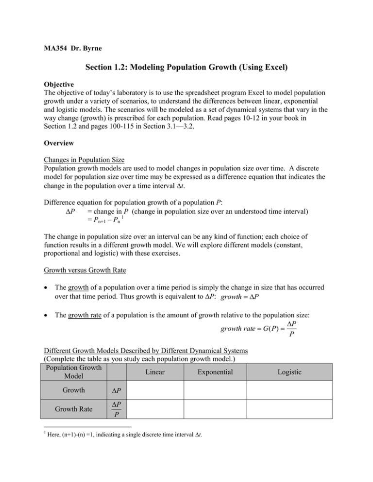
MA354 Dr. Byrne
Section 1.2: Modeling Population Growth (Using Excel)
Objective
The objective of today’s laboratory is to use the spreadsheet program Excel to model population
growth under a variety of scenarios, to understand the differences between linear, exponential
and logistic models. The scenarios will be modeled as a set of dynamical systems that vary in the
way change (growth) is prescribed for each population. Read pages 10-12 in your book in
Section 1.2 and pages 100-115 in Section 3.1—3.2.
Overview
Changes in Population Size
Population growth models are used to model changes in population size over time. A discrete
model for population size over time may be expressed as a difference equation that indicates the
change in the population over a time interval t.
Difference equation for population growth of a population P:
P
= change in P (change in population size over an understood time interval)
= Pn+1 – Pn 1
The change in population size over an interval can be any kind of function; each choice of
function results in a different growth model. We will explore different models (constant,
proportional and logistic) with these exercises.
Growth versus Growth Rate

The growth of a population over a time period is simply the change in size that has occurred
over that time period. Thus growth is equivalent to P: growth  P

The growth rate of a population is the amount of growth relative to the population size:
P
growth rate  G( P) 
P
Different Growth Models Described by Different Dynamical Systems
(Complete the table as you study each population growth model.)
Population Growth
Linear
Exponential
Model
1
Growth
P
Growth Rate
P
P
Here, (n+1)-(n) =1, indicating a single discrete time interval t.
Logistic
Exercise 1: Linear Growth Model – Growth is Independent of Population Size
Suppose that the change in population size over a time interval is always the same fixed value (a
constant). In this case, the change in population size doesn’t depend upon anything, as it is fixed.
We describe this model with the difference equation P = k where k is the constant growth over
a fixed, understood time interval.
P = k
1. Build the model: Build a dynamical system in an Excel workbook that models linear growth
(i.e., using P = k). Let the initial population size P0 and value of k be free parameters in the
model. Consider the growth and the growth rate:
Growth =
Growth Rate =
Meaning of k? ________________________
2. Implementing the Model for Specific Parameters: Suppose that the initial size of the
population is 60 (P0 = 60) Plot the population size verses time over 20 time intervals for the
following values of k:
(a) 𝑘 = 3
(b) 𝑘 = 0
(c) 𝑘 = −1
Group Project: Fitting Hypothetically Linear Growth Data (sort as A-alphas)
Discussion: A scientist presents you with the following data for the number of specimens of an
invasive species counted over a week in a given square acre. Assuming first that the growth is
noisy (stochastic) but can be approximated using a linear model, estimate the growth constant k.
# Specimens Found per Day
D1
D2
D3
D4
D5
D6
D7
1
2
4
9
14
16
23
k ≈ _____________
Do you think that the population growth is described well by a linear model? Why or why not?
What do you estimate is your confidence or the degree of accuracy in your estimation of the
parameter k? Assume you are a post-doc for a scientist that would like to estimate how many
specimens there will be on Day 14. Suggest a prediction with a range that factors in your current
confidence regarding k.
Prediction = [min likely value, max likely value] =
The scientist would like a more precise measure of k and asks if more data points would
help. She wants to know if you would like more frequent data points, or data points over a longer
interval. How should you answer?
Exercise 2: Proportional Growth Model – Exponential Model
In exponential growth, growth depends upon the population size:
P = k * P
1. Build and implement the model: Use Excel to model the population growth described by
exponential growth. Copy your Excel worksheet for linear growth into a new worksheet and
modify the equations to reflect exponential growth. As before, include a graph that shows the
population size for 20 time intervals, where the initial population size P0 and value of k are
free parameters. (For the initial model implementation, set P0 = 60 and k=0.3.)
Growth =
Growth Rate =
Meaning of k? ________________________
Group Project: Fitting Hypothetically Exponential Growth Data (sort as A-alphas)
Discussion: The same scientist has collected one more week of data. He no longer believes the
growth is linear. Assuming first that the growth is noisy (stochastic) but can be approximated
using an exponential growth model, estimate the growth constant k.
# Specimens Found per Day, Second Week
D8
31
D9
41
D10
51
D11
61
D12
74
D13
86
D14
99
k ≈ _____________
Do you think that the population growth is described well by an exponential model? Why or why
not?
Given your confidence or the degree of accuracy in your estimation of the parameter k, provide a
prediction for Day 21:
Exercise 3: Biologically Motivated Growth Model (Deriving the Logistic Growth Model)
Although there are some examples in biology of linear and exponential growth, growth and
growth rate are both usually size dependent. This is true over a range of scales, from bacteria
populations to tumors to whole organisms. On the one hand, the amount of growth over a fixed
interval is often proportional to size. On the other hand, the growth rate is often inversely
proportional to size: the growth rate is fastest when the population is small and slowest when the
population is large. (Due, for example, to resource management and availability.)
In this exercise, we will build a model for a scenario where the growth rate depends upon the
population size in the following ways:

When the population is small, the growth rate is a maximal growth rate k. In particular, in
the limit of a vanishingly small population size, the growth rate is k:
P = kP when P = 0.

When the population is a maximal size M (the carrying capacity), the growth rate is zero:
P = 0P when P = M.
In this simple scenario, the growth rate depends upon
the population size. In other words, the growth rate is a
function of P. The two assumptions above provide two
points for this function, at the limits when P is minimal
and maximal. The two points are shown on the plot
below.
1. We want to functionally describe the growth rate as a function of the population size. The
simplest continuous function (let’s call it PGRB) that passes through these two points in a line.
Sketch this line on the plot above and write the equation in terms of k, P and M:
Growth rate = PGRB =
2. Given a population growth rate PGRB, we have ∆𝑃 = 𝑃𝐺𝑅𝐵 ∗ 𝑃. Write down the difference
equation for growth of the population:
Growth = ∆𝑃 = 𝑃𝐺𝑅𝐵 ∗ 𝑃
3. Build the model: Use Excel to model the population growth described by ∆𝑃 = 𝑃𝐺𝑅𝐵 ∗ 𝑃.
Include a graph for the population size verses time for 20 time intervals, given the initial
population size is P0 = 60, k=0.3 and M = 300.
Exercise 4: Logistic Growth
The function GB(P) in the previous exercise was chosen as
the simplest function that yielded a maximal growth rate of
k at small pop sizes and a minimal growth rate of 0 at the
maximal population size M. Obviously, this function can
vary in different ways between points as a monotonically
decreasing function. For example, we can imagine that the
growth rate changes slowly at first or quickly at first:
Each different function represents a different growth model that may or may not be a better
description of growth in a real-world scenario. Model construction is largely concerned with
finding the function which is most descriptive for a particular problem.
In your book, the difference equation for logistic population growth is written as:
P = k (M – P)*P
(page 407, Eqn 11.9)
1. Build the model: Use Excel to model the population growth described by logistic growth.
Include a graph for the population size verses time for 50 time intervals, given the initial
population size is P0 = 60, k=0.0005 and M = 500. Notice that the population size initially
changes fast (exponential growth) and then changes slowly (logarithmic growth).
2. For the logistic growth equation, solve for the population growth rate of the logistic function
(let’s call it PGRL) given that ∆𝑃 = 𝑃𝐺𝑅𝐿 ∗ 𝑃.
PGRL =
3. How does the function PGRL used to describe the logistic growth rate compare with your
function PGRB? In particular, what is the ratio PGRB / PGRL?
4. The logistic function can be modeled in equivalent ways:
P = k1 (M – P)*P = k2 (1 – P/M)*P
Convince yourself these two equations are similar up to the parameters k1 and k2. What is the
relationship between k1 and k2?
Exercise 5: Relationships Between Models
1. Note that logistic growth is exponential when the population size is small. In particular, the
growth is exponential when the population size is farthest from the carrying capacity. Derive
the equation for exponential growth from the logistic equation for growth by considering the
limit as M approaches infinity. (Hint: use the form of the equation from Exercise 3 rather
than Exercise 4.)
2. Each of the models (linear, exponential, logistic) has been described with a free parameter k.
Compare the k in these three models. Do they represent the same thing?
Model
Growth
Growth Rate
Meaning of k
Linear
Exponential
Logistic
(either version)
3. Only the logistic model explicitly mentions M, the carrying capacity. What would M be for
the linear and exponential models?
Some other growth models found in the literature:
𝑘2

Gompertzian Growth: ∆𝑃 = 𝑘1 ln (

Mitscherlich model: ∆𝑃 = 𝑘2 (𝑘1 − 𝑃(𝑡)) (crop models, historically)

Inverse polynomial: ∆𝑃 = 𝑘2 (𝑘1 − 𝑃(𝑡)) (crop models, historically)
𝑃(𝑡)
) 𝑃(𝑡) (tumor growth)
2