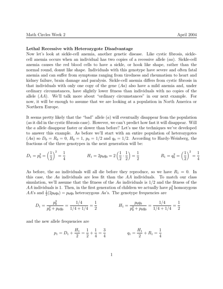
Math Circles Week 2
April 2004
Lethal Recessive with Heterozygote Disadvantage
Now let’s look at sickle-cell anemia, another genetic disease. Like cystic fibrosis, sicklecell anemia occurs when an individual has two copies of a recessive allele (aa). Sickle-cell
anemia causes the red blood cells to have a sickle, or hook like shape, rather than the
normal round, donut like shape. Individuals with this genotype have severe and often fatal
anemia and can suffer from symptoms ranging from tiredness and rheumatism to heart and
kidney failure, brain damage and paralysis. Sickle-cell anemia differs from cystic fibrosis in
that individuals with only one copy of the gene (Aa) also have a mild anemia and, under
ordinary circumstances, have slightly lower fitness than individuals with no copies of the
allele (AA). We’ll talk more about “ordinary circumstances” in our next example. For
now, it will be enough to assume that we are looking at a population in North America or
Northern Europe.
It seems pretty likely that the “bad” allele (a) will eventually disappear from the population
(as it did in the cystic fibrosis case). However, we can’t predict how fast it will disappear. Will
the a allele disappear faster or slower than before? Let’s use the techniques we’ve developed
to answer this example. As before we’ll start with an entire population of heterozygotes
(Aa) so D0 = R0 = 0, H0 = 1, p0 = 1/2 and q0 = 1/2. According to Hardy-Weinberg, the
fractions of the three genotypes in the next generation will be:
D1 = p20 =
2
1
2
=
1
4
H1 = 2p0 q0 = 2
1
1 1
=
·
2 2
2
R1 = q02 =
2
1
2
=
As before, the aa individuals will all die before they reproduce, so we have R1 = 0. In
this case, the Aa individuals are less fit than the AA individuals. To match our class
simulation, we’ll assume that the fitness of the Aa individuals is 1/2 and the fitness of the
AA individuals is 1. Then, in the first generation of children we actually have p20 homozygous
AA’s and 21 (2p0 q0 ) = p0 q0 heterozygous Aa’s. The genotype frequencies are
D1 =
p20
1/4
1
=
=
2
p0 + p0 q0
1/4 + 1/4
2
H1 =
p20
p0 q0
1/4
1
=
=
+ p0 q0
1/4 + 1/4
2
and the new allele frequencies are
p 1 = D1 +
1 1
3
H1
= + =
2
2 4
4
q1 =
1
H1
1
+ R1 =
2
4
1
4
Math Circles Week 2
April 2004
We already notice that things seem to be happening faster. In our cystic fibrosis example
p1 = 2/3 and p2 = 3/4. Now, we have p1 = 3/4 in just one step. Let’s see what happens
after one more generation.
p21
3
(3/4)2
=
=
2
2
p1 + p1 q1
4
(3/4) + (3/4) (1/4)
1
(3/4) (1/4)
p1 q1
=
=
H2 = 2
2
p1 + p1 q1
4
(3/4) + (3/4) (1/4)
D2 =
p 2 = D2 +
3 1
7
H2
= + =
2
4 8
8
q2 =
H2
1
+ R2 =
2
8
In this generation, the fraction of a alleles has decreased from 1/4 to 1/8 and the fraction of
A alleles seems to be increasing towards 1. Will the fraction of A alleles actually go to 1?
Let’s go through the same analysis as before.
Let’s switch to the more general case where p0 is not specified from the start. Like before,
we can use our general result to look at our class simulation by setting p0 = 1/2. First, we
write down a general equation for p1 remembering that q0 = 1 − p0 .
p 1 = D1 +
p2
p0 q0 /2
p0 (2p0 + 1 − p0 ) /2
(p0 + 1)/2
1
H1
= 2 0
+ 2
=
=
= (p0 + 1)
2
p0 + p0 q0 p0 + p0 q0
p0 (p0 + 1 − p0 )
1
2
This formula will hold in general for any step so we can write
1
pn+1 = (pn + 1)
2
Let’s solve for the equilibrium points, p∗ . We have
1
p∗ = (p∗ + 1) ⇒ 2p∗ = p∗ + 1 ⇒ p∗ = 1
2
As before, the only equilibrium point is p∗ = 1, or the case when A is the only allele in the
population. Will the population actually go to this equilibrium? Our first few calculations
suggested that the population will.
Let’s see if we can come up with a formula for pn in terms of p0 . Do you see a pattern in what
we’ve calculated so far for the p0 = 1/2 case? We have p0 = 1/2, p1 = 3/4 and p2 = 7/8. A
2
Math Circles Week 2
April 2004
general formula doesn’t jump out quite as easily as before. Let’s try looking at the first few
iterations of the general case and see if that helps.
1
1
p1 = p0 +
2
2 1 1
1
1
1 1
1
p0 + + 1 = p0 +
+
p2 = (p1 + 1) =
2
2 2
2
4
4 2
1
1 1
1 1
1 1 1
1
+ 1 = p0 +
p0 +
+
+ +
p3 = (p2 + 1) =
2
2 4
4 2
8
8 4 2
It looks like
1
1
1
1
pn = n p0 + n + n−1 + · · · +
2
2
2
2
might be what we are looking for. Remembering that
1 1 1
+ + +··· = 1
2 4 8
1 1
1
1
+ +···+ n = 1− n
2 4
2
2
and
we have
1
1
pn = n p0 + 1 − n
2
2
=
1
1
(p0 − 1) + 1 = 1 − n (1 − p0 )
n
2
2
Again, we can use induction to prove that this is the correct formula. First, we notice that
the formula gives us the correct answer when n = 1.
1
1 1
1
p1 = 1 − (1 − p0 ) = 1 − + p0 = (1 + p0 )
2
2 2
2
Let’s assume it is correct for n = k and show that it works for n = k + 1.
pk+1
1
1
1
1
1
1
1
1 − k (1 − p0 ) + 1 = − k+1 (1 − p0 ) + = 1 − k+1 (1 − p0 )
= (pk + 1) =
2
2
2
2 2
2
2
This is exactly the form our formula predicts. Now, we can use our formula for pn to predict
what will happen after a long time has passed. As n → ∞, the fraction 1/2n → 0. Therefore,
pn → 1 as expected.
3
Math Circles Week 2
April 2004
As in the cystic fibrosis example the “bad” allele will eventually disappear, but will it disappear faster or slower? Let’s go back to our specific example with p0 = 1/2 and make a table
of values. For comparison, we’ll include our results from before.
|| p0
||
AA = Aa || 0.5
||
AA > Aa || 0.5
p1
p2
p3
p4
p5
···
p10
p20
0.667
0.750
0.8000
0.83333
0.857143
···
0.9167
0.95
0.75
0.875
0.9375
0.96875
0.984375
···
0.9990
1.0
The second example seems to be approaching one must faster. This makes sense as there is
a disadvantage to having any a’s at all. Let’s look at qn like we did before.
qn = 1 − pn == 1 − 1 +
1
1
(1
−
p
)
=
(1 − p0 )
0
2n
2n
From this equation, we see that qn (the fraction of allele a in the population) approaches
zero at a rate related to 2n which is exponential. In our cystic fibrosis example this rate was
related to n. Hopefully, it is obvious that in the second example the a allele will disappear
much, much faster than in the first example.
To summarize, we’ve found that if a recessive allele is lethal when it occurs as a homozygote
(aa), it will eventually disappear from the population. If the heterozygote (Aa) is also
detrimental, the rate of disappearance will be much faster.
Lethal Recessive with Heterozygote Advantage
Now, we’d like to return to an idea mentioned in the introduction to our sickle-cell anemia
example. That is, we said that under ordinary circumstances, heterozygous individuals (Aa)
are slightly less fit than dominant homozygous (AA) individuals. What exactly is meant
by “ordinary circumstances”? It turns out that in regions of Africa that have high levels
of (falciparum) malaria, the heterozygous genotype (Aa) actually has higher fitness than
the normal homozygotes (AA). In this case, the slight abnormalities in the red blood cells
caused by anemia actually protect a person from malaria. In a place like Africa, where large
numbers of people suffer from malaria at some point in their lives, it is actually better (in
terms of fitness) to suffer slightly from anemia, as it provides protection from the more lethal
malaria. In general, we call this type of situation heterozygote advantage.
What will happen in this situation? Will the detrimental allele a still disappear, and if
so, how fast? As before we’ll start with an entire population of heterozygotes (Aa) so
4
Math Circles Week 2
April 2004
D0 = R0 = 0, H0 = 1, p0 = 1/2 and q0 = 1/2. Hardy-Weinberg gives us the fractions of the
three genotypes in the next generation:
D1 =
p20
2
1
=
2
1
1 1
=
H1 = 2p0 q0 = 2
·
2 2
2
1
=
4
R1 =
q02
=
2
1
2
=
The aa individuals will all die as before, but in this case, the AA individuals are less fit than
the Aa individuals. To match our class simulation, we’ll assume that the fitness of the AA
individuals is 1/2 and the fitness of the Aa individuals is 1. Then, in the first generation of
children we actually have p20 /2 homozygous AA’s and 2p0 q0 heterozygous Aa’s. The genotype
frequencies are
D1 =
1/8
1
p20 /2
=
=
2
p0 /2 + 2p0 q0
1/8 + 1/2
5
H1 =
1/2
2p0 q0
4
=
=
+ 2p0 q0
1/8 + 1/2
5
p20 /2
and the new allele frequencies are
p 1 = D1 +
1 2
3
H1
= + =
2
5 5
5
q1 =
H1
2
+ R1 =
2
5
The frequency of the A allele increased, but not by much. Let’s see what happens after a
few more generations.
9
p21 /2
(3/5)2 /2
3
=
=
=
2
2
p1 /2 + 2p1 q1
33
11
(3/5) /2 + 2 (3/5) (2/5)
2p1 q1
24
2 (3/5) (2/5)
8
H2 = 2
=
=
=
2
p1 /2 + 2p1 q1
33
11
(3/5) /2 + 2 (3/5) (2/5)
D2 =
p 2 = D2 +
3
4
7
H2
=
+
=
2
11 11
11
q2 =
H2
4
+ R2 =
2
11
49
(7/11)2 /2
7
p22 /2
=
=
=
2
2
p2 /2 + 2p2 q2
161
23
(7/11) /2 + 2 (7/11) (4/11)
2 (7/11) (4/11)
112
16
2p2 q2
=
=
=
H3 = 2
2
p2 /2 + 2p2 q2
161
23
(7/11) /2 + 2 (7/11) (4/11)
D3 =
p 3 = D3 +
H3
7
8
15
=
+
=
2
23 23
23
q3 =
5
H3
8
+ R2 =
2
23
1
4
Math Circles Week 2
April 2004
The frequency of the A allele doesn’t seem to be going to 1 in this example or, if it is, it is
moving very slowly.
Let’s go ahead and look at the more general case with p0 as a variable. A general equation
for p1 is
p20 /2
2p0 q0 /2
p0 (p0 + 2 − 2p0 ) /2
2 − p0
H1
= 2
+ 2
=
=
p 1 = D1 +
2
p0 /2 + 2p0 q0 p0 /2 + 2p0 q0
p0 (p0 + 4 − 4p0 ) /2
4 − 3p0
In general, we have
pn+1 =
2 − pn
4 − 3pn
Let’s solve for the equilibrium points, p∗ . We have
p∗ =
2 − p∗
⇒ 4p∗ − 3(p∗ )2 = 2 − p∗ ⇒ 3(p∗ )2 − 5p∗ + 2 = 0 ⇒ (3p∗ − 2)(p∗ − 1) = 0
4 − 3p∗
In this case there are two equilibrium points p∗ = 2/3 and p∗ = 1. Which equilibrium will
the population go to? Our calculations seem to be heading towards the first equilibrium,
but how can we be sure? Let’s see if we can write down a general formula for pn .
p1 =
2 − p0
4 − 3p0
2−p0
2 − 4−3p
2 − p1
6 − 5p0
8 − 6p0 − 2 + p0
0
=
p2 =
=
=
2−p
4 − 3p1
16 − 12p0 − 6 + 3p0
10 − 9p0
4 − 3 4−3p00
6−5p0
2 − 10−9p
14 − 13p0
2 − p2
20 − 18p0 − 6 + 5p0
0
=
=
=
p3 =
6−5p
4 − 3p2
40 − 36p0 − 18 + 15p0
22 − 21p0
4 − 3 10−9p00
Can you figure out a general formula? In this case its pretty hard to get the right form,
so we’ll use another method to study the dynamics. We can plot a graph of our iterative
formula
pn+1 =
2 − pn
4 − 3pn
6
Math Circles Week 2
April 2004
with pn as the x-axis and pn+1 as the y-axis and use a method called cobwebbing to evaluate
the long term dynamics. At the same time, we’ll make plots of our previous models and see
how our results compare to the cobweb diagrams.
Looking at a graph of the iteration function, we see that if we draw a vertical line starting
at p0 on the x-axis, and stop when we hit the iteration function, we will be at a height of
p1 . For the next iteration, we want to start at p1 on the x-axis. We can make this easy by
drawing a second line on the graph corresponding to the function y = x or pn = pn+1 . Now,
starting at the height of p1 , we draw a horizontal line until we intersect the line y = x. This
point will correspond to a value of p1 on the x-axis. Now, draw a vertical line from this point
until we intersect the iteration function again. This will give us the next allele frequency. We
can continue this process indefinitely. After a few iterations, we will notice that we seem to
be moving closer and closer to a point where the iteration function intersects the line y = x.
This intersection point is an equilibrium point.
The cobwebbing procedure for our iteration function predicts that if, at the start, there is at
least one allele of each type, the A allele will eventually be present in 2/3 of the population
and the a allele will eventually be present in 1/3. So, even though the a allele is pretty bad
when it occurs alone, the fact that it can do some good in combination with the A allele
allows it to survive in the population.
It turns out that the general formula for pn is
pn =
1
+ 2 − 23n (1 − p0 )
2n
1
1
+
3
1
−
(1 − p0 )
n
n
2
2
=
1 + (2n+1 − 3)(1 − p0 )
1 + 3(2n − 1)(1 − p0 )
As n → ∞, the fraction 1/2n → 0. Therefore,
pn →
2
2(1 − p0 )
=
3(1 − p0 )
3
This matches the prediction from our cobwebbing picture.
Unlike the previous two examples, the “bad” allele does not disappear. How fast will the
7
Math Circles Week 2
April 2004
population approach the equilibrium point? Let’s add one more row to our table.
||
||
AA = Aa ||
||
AA > Aa ||
||
AA < Aa ||
p0
p1
p2
p3
p4
p5
···
p10
p20
0.5
0.667
0.750
0.8000
0.83333
0.857143
···
0.9167
0.95
0.5
0.750
0.875
0.9375
0.96875
0.984375
···
0.9990
1.0
0.5
0.600
0.636
0.6522
0.65957
0.663158
···
0.6666
0.667
The good allele A seems to converge pretty fast to the 2/3 equilibrium. Let’s look at qn like
we did before.
qn = 1 − pn = 1 −
1 + 3(2n − 1)(1 − p0 ) − 1 − (2n+1 − 3)(1 − p0 )
1 + (2n+1 − 3)(1 − p0 )
=
1 + 3(2n − 1)(1 − p0 )
1 + 3(2n − 1)(1 − p0 )
=
[3(2n ) − 3 − 2n+1 + 3] (1 − p0 )
=
1 + 3(2n − 1)(1 − p0 )
=
1
2n
(3 − 2)(1 − p0 )
+ 3(1 − p0 ) − 23n (1 − p0 )
1 − p0
=
3(1 − p0 ) + 21n (1 − 3(1 − p0 ))
3+
1
1
2n
3p0 −2
1−p0
From this equation, we see that qn (the fraction of allele a in the population) approaches
1/3 at a rate related to 2n which is exponential and fairly rapid.
In summary, we’ve found that if a recessive allele is lethal when it occurs as a homozygote
(aa), it will eventually disappear from the population. If the heterozygote (Aa) is also
detrimental, the rate of disappearance will be much faster. However, if the heterozygote
(Aa) is beneficial, the bad a allele will never disappear.
Extra Problems
(1) In the human population there are four blood types: A, B, O and AB. These blood
groups are caused by three alleles: I A , I B and I O . Individuals with genotypes I A I A and
I A I O have blood type A, those with I B I B and I B I O have blood type B, those with I A I B
have blood type AB, and those with I O I O have type O.
(a) If p is the fraction of I A alleles in the population, q is the fraction of I B alleles, and r
is the fraction of I O alleles, find the Hardy-Weinberg equilibrium proportions for the four
blood types A, B, AB and O.
(b) If p = q = r = 1/3, what are the proportions of each blood type in the population?
8
Math Circles Week 2
April 2004
(2) For the examples done in class, we assumed that fitness values were 0, 1/2 or 1. What if
in our sickle-cell anemia/ malaria example, the fitness of AA individuals is only slightly less
than that of Aa individuals? Will we get the same result? Let Aa individuals have a fitness
of 1, AA individuals have a fitness of (1 − s) and aa individuals have a fitness of 0.
(a) Find a formula for pn+1 as a function of pn .
(b) Find the equilibrium points.
(c) Find a general formula for pn as a function of p0 . It may be helpful to let α = 1 + s and
β = 1 − s. Also, notice that
1 + β + · · · β n−1 =
1 − βn
1−β
(d) Make a table of p for the case s = 0.01. How fast does the population go to its equilibrium? Is it similar to the case when s = 0?
References
Davis, Tom. Mathematical Biology, 1999. http://www.geometer.org/mathcircles
Futuyma, Douglas. Evolutionary Biology, 1998. Sinauer Associates, Inc., Massachusetts.
Griffiths, A., Miller, J. Suzuki, D. Lewontin, R. and Gelbart, W. An Introduction to Genetic
Analysis, 6th Ed., 1996. W. H. Freeman and Company, New York.
Hartl, Daniel. A Primer of Population Genetics, 3rd Ed., 2000. Sinauer Associates, Inc.,
Massachusetts.
9