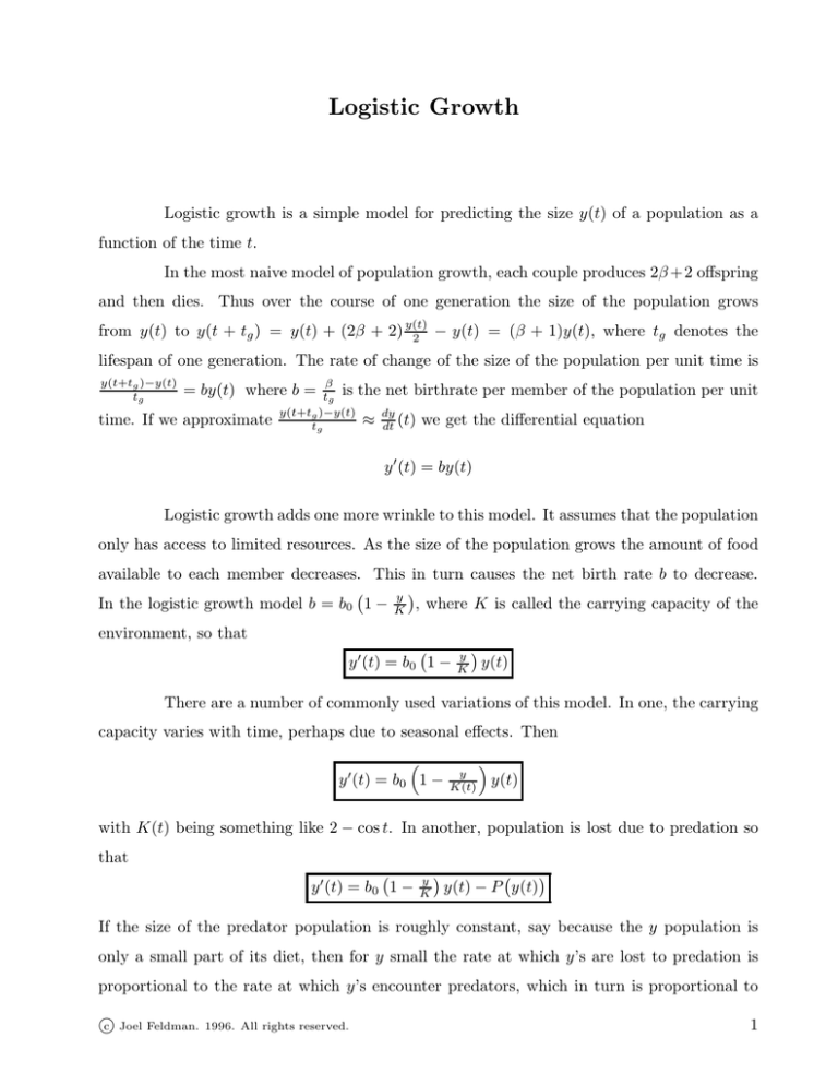
Logistic Growth
Logistic growth is a simple model for predicting the size y(t) of a population as a
function of the time t.
In the most naive model of population growth, each couple produces 2β +2 offspring
and then dies. Thus over the course of one generation the size of the population grows
− y(t) = (β + 1)y(t), where tg denotes the
from y(t) to y(t + tg ) = y(t) + (2β + 2) y(t)
2
lifespan of one generation. The rate of change of the size of the population per unit time is
y(t+tg )−y(t)
tg
β
tg is the net birthrate per member of the population
y(t+tg )−y(t)
≈ dy
(t) we get the differential equation
tg
dt
= by(t) where b =
time. If we approximate
per unit
y ′ (t) = by(t)
Logistic growth adds one more wrinkle to this model. It assumes that the population
only has access to limited resources. As the size of the population grows the amount of food
available to each member decreases. This in turn causes the net birth rate b to decrease.
y
In the logistic growth model b = b0 1 − K
, where K is called the carrying capacity of the
environment, so that
y ′ (t) = b0 1 −
y
K
y(t)
There are a number of commonly used variations of this model. In one, the carrying
capacity varies with time, perhaps due to seasonal effects. Then
y ′ (t) = b0 1 −
y
K(t)
y(t)
with K(t) being something like 2 − cos t. In another, population is lost due to predation so
that
y ′ (t) = b0 1 −
y
K
y(t) − P y(t)
If the size of the predator population is roughly constant, say because the y population is
only a small part of its diet, then for y small the rate at which y’s are lost to predation is
proportional to the rate at which y’s encounter predators, which in turn is proportional to
c Joel Feldman.
1996. All rights reserved.
1
y(t). When y is large the rate at which y’s are lost to predation becomes a constant because
the predators don’t want to eat any more y’s. A predation function which has this behaviour
is
P (y) =
c Joel Feldman.
1996. All rights reserved.
αy
1+γy
2