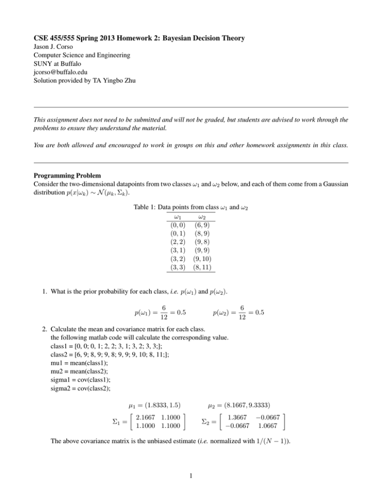
CSE 455/555 Spring 2013 Homework 2: Bayesian Decision Theory
Jason J. Corso
Computer Science and Engineering
SUNY at Buffalo
jcorso@buffalo.edu
Solution provided by TA Yingbo Zhu
This assignment does not need to be submitted and will not be graded, but students are advised to work through the
problems to ensure they understand the material.
You are both allowed and encouraged to work in groups on this and other homework assignments in this class.
Programming Problem
Consider the two-dimensional datapoints from two classes ω1 and ω2 below, and each of them come from a Gaussian
distribution p(x|ωk ) ∼ N (µk , Σk ).
Table 1: Data points from class ω1 and ω2
ω1
ω2
(0, 0) (6, 9)
(0, 1) (8, 9)
(2, 2) (9, 8)
(3, 1) (9, 9)
(3, 2) (9, 10)
(3, 3) (8, 11)
1. What is the prior probability for each class, i.e. p(ω1 ) and p(ω2 ).
p(ω1 ) =
6
= 0.5
12
p(ω2 ) =
6
= 0.5
12
2. Calculate the mean and covariance matrix for each class.
the following matlab code will calculate the corresponding value.
class1 = [0, 0; 0, 1; 2, 2; 3, 1; 3, 2; 3, 3;];
class2 = [6, 9; 8, 9; 9, 8; 9, 9; 9, 10; 8, 11;];
mu1 = mean(class1);
mu2 = mean(class2);
sigma1 = cov(class1);
sigma2 = cov(class2);
µ1 = (1.8333, 1.5)
2.1667 1.1000
Σ1 =
1.1000 1.1000
µ2 = (8.1667, 9.3333)
1.3667 −0.0667
Σ2 =
−0.0667 1.0667
The above covariance matrix is the unbiased estimate (i.e. normalized with 1/(N − 1)).
1
3. Derive the equation for the decision boundary that separates these two classes, and plot the boundary.
(Hint: you may want to use the posterior probability p(ω1 |x))
p(ωi |x) ∝ p(x|ωi )p(ωi )
For minimum error rate classification, we can write the discriminant function for each class as
gi (x) = p(x|ωi )p(ωi )
since this question involves Gaussian distribution, apply natural logrithm will make it easier for us, i.e. we
can write the discriminant function as
gi (x) = ln p(x|ωi ) + ln p(ωi )
so the discriminant function in this case would be
1
1
ln |Σi | + ln p(ωi )
gi (x) = − (x − µi )T Σ−1
i (x − µi ) − ln 2π −
2
2
The decision boundary would be the solution of g1 (x) = g2 (x).
The following code implements the above
syms x1 x2;
g1 = -0.5*([x1;x2]-mu1’)’*inv(sigma1)*([x1;x2]-mu1’)-log(2*pi)-0.5*log(det(sigma1));
g2 = -0.5*([x1;x2]-mu2’)’*inv(sigma2)*([x1;x2]-mu2’)-log(2*pi)-0.5*log(det(sigma2));
g = g1 - g2;
ezplot(g, [[-1,11], [-1,11]]);
Term ln p(ωi ) is omitted since we have equal prior in this problem. The ploted boundary looks like the following
2
4. Think of the case that the penalties for misclassification are different for the two classes (i.e. not zero-one
loss), will it affect the decision boundary, and how?
Let’s consider the case that misclassify a sample to class 2 cost more than misclassify a sample to class 1.
Then the decision boundary will move toward class 2, i.e. more samples will be classified as class 1. Since we
can afford more errors in the case that we misclassify samples to class 1.
Mathematical Problem
Consider two classes ω1 and ω2 in pattern space Ω with continuous probability distribution p1 (x) and p2 (x), respectively. This two-class classification problem can be interpreted as dividing space Ω into two exhaustive and disjoint
sets Ω1 and Ω2 , such that Ω1 ∪ Ω2 = Ω and Ω1 ∩ Ω2 = ∅. If xi ∈ Ωk then assign xi to class ωk .
1. Suppose you are given a discriminant function f (·), list the two errors this function can make.
n ω , whenx ∈ ω
2
1
f (x) =
ω1 , whenx ∈ ω2
2. Write down the probability of error corresponds to the two erros.
Z
Z
p1 (x)dx
and
p2 (x)dx
Ω2
Ω1
3. Suppose the costs for the two types of errors are c1 and c2 , write down the total expected cost.
Assume that c1 is the cost of the first error and c2 is the cost of the second error. Then the expected cost would
be
Z
Z
c1 p(ω1 )
p1 (x)dx + c2 (1 − p(ω1 ))
p2 (x)dx
Ω2
Ω1
3