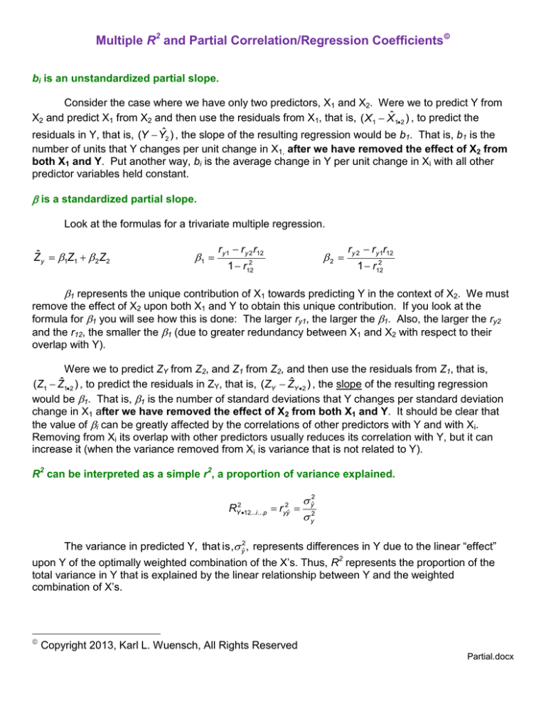
Multiple R2 and Partial Correlation/Regression Coefficients
bi is an unstandardized partial slope.
Consider the case where we have only two predictors, X1 and X2. Were we to predict Y from
X2 and predict X1 from X2 and then use the residuals from X1, that is, ( X 1  Xˆ 12 ) , to predict the
residuals in Y, that is, (Y  Yˆ ) , the slope of the resulting regression would be b1. That is, b1 is the
2
number of units that Y changes per unit change in X1, after we have removed the effect of X2 from
both X1 and Y. Put another way, bi is the average change in Y per unit change in Xi with all other
predictor variables held constant.
 is a standardized partial slope.
Look at the formulas for a trivariate multiple regression.
Zˆ y  1Z1   2 Z2
1 
r y 1  r y 2 r12
2 
1  r122
r y 2  r y 1r12
1  r122
1 represents the unique contribution of X1 towards predicting Y in the context of X2. We must
remove the effect of X2 upon both X1 and Y to obtain this unique contribution. If you look at the
formula for 1 you will see how this is done: The larger ry1, the larger the 1. Also, the larger the ry2
and the r12, the smaller the 1 (due to greater redundancy between X1 and X2 with respect to their
overlap with Y).
Were we to predict ZY from Z2, and Z1 from Z2, and then use the residuals from Z1, that is,
ˆ
(Z1  Z12 ) , to predict the residuals in ZY, that is, (ZY  ZˆY 2 ) , the slope of the resulting regression
would be 1. That is, 1 is the number of standard deviations that Y changes per standard deviation
change in X1 after we have removed the effect of X2 from both X1 and Y. It should be clear that
the value of i can be greatly affected by the correlations of other predictors with Y and with Xi.
Removing from Xi its overlap with other predictors usually reduces its correlation with Y, but it can
increase it (when the variance removed from Xi is variance that is not related to Y).
R2 can be interpreted as a simple r2, a proportion of variance explained.
2
Y 12...i ...p
R
 y2ˆ
r  2
y
2
yyˆ
The variance in predicted Y, that is, ŷ2, represents differences in Y due to the linear “effect”
upon Y of the optimally weighted combination of the X’s. Thus, R2 represents the proportion of the
total variance in Y that is explained by the linear relationship between Y and the weighted
combination of X’s.

Copyright 2013, Karl L. Wuensch, All Rights Reserved
Partial.docx
R2 can be obtained from beta weights and zero-order correlation coefficients.
RY212...i ...p    i r yi    i2  2  i  j r ij
2
(i  j)
The sum of the squared beta weights represents the sum of the unique contributions of the predictors
while the rightmost term represents the redundancy among the predictors.
R y212 
rY21  rY22  2rY 1rY 2 r12
1  r122
  1rY 1   2 rY 2
Note that in determining R2 we have added together the two bivariate coefficients of
determination and then corrected (reduced) that sum for the redundancy of X1 and X2 in predicting Y.
Squared correlation coefficients represent proportions of variance explained.
a+b+c+d=1
rY21  b  c
sr12 
b
b
(a  b  c  d )  1
rY22  d  c
r122  c  e
RY212  b  c  d
c = redundancy (aka commonality)
A squared semipartial correlation represents the proportion of all the variance in Y that is
associated with one predictor but not with any of the other predictors. That is, in terms of the Venn
diagram,
sr12 
b
 b.
(a  b  c  d )  1
The squared semipartial can also be viewed as the decrease in R2 that results from removing
a predictor from the model, that is,
sri 2  RY212...i ...p  RY212...(i )...p
In terms of residuals, the semipartial correlation for Xi is the r between all of Y and Xi from
which the effects of all other predictors have been removed. That is,
sr1  corr betweenY and ( X1  Xˆ 12 )
3
A squared partial correlation represents a fully partialled proportion of the variance in Y: Of
the variance in Y that is not associated with any other predictors, what proportion is associated with
the variance in Xi. That is, in terms of the Venn diagram,
pr12 
b
ab
The squared partial can be obtained from the squared semipartial:
sri 2
pri 
1  RY212...(i )... p
2
pri 2  sri 2
The (i) in the subscript indicates that Xi is not included in the R2.
In terms of residuals, the partial correlation for Xi is the r between Y from which all other
predictors have been partialled and Xi from which all other predictors have been removed. That is,
pr1  corr between(Y  Yˆ2 ) and ( X1  Xˆ 12 )
If the predictors are well correlated with one another, their partial and semipartial coefficients
may be considerably less impressive than their zero-order coefficients. In this case it might be helpful
to conduct what some call a commonality analysis. In such an analysis one can determine how much
of the variance in Y is related to the predictors but not included in the predictors partial or semipartial
coefficients. For the Venn diagram above, that is area c. For more details, please see my document
Commonality Analysis.
A demonstration of the partial nature of multiple correlation and regression coefficients.
Run the program Partial.sas from my SAS programs page. The data are from an earlier
edition of Howell (6th edition, page 496). Students at a large university completed a survey about
their classes. Most of the questions had a five-point scale where “1” indicated that the course was
lousy and “5” indicated that it was great. The variables in the data set are:
 Overall: the overall quality of the lectures in the class
 Teach: the teaching skills of the instructor
 Exam: the quality of the tests and exams
 Knowledge: how knowledgeable the instructor was
 Grade: the grade the student expected to receive (1 = F, …, 5 = A)
 Enroll: the number of students in the class.
The data represent a random sample from the population of classes. Each case is from one
class.
Look at the data step. Here I create six Z scores, one for each of the variables in the model.
The first invocation of Proc Reg does a multiple regression predicting Overall from the five
predictor variables. SCORR2 tells SAS I want squared semipartial correlation coefficients. PCORR2
requests squared partial correlation coefficients. TOL requests tolerances. STB tells SAS I want
4
Beta weights. If you look at the output, you will see that I have replicated the results reported in
Howell. “Parameter Estimates” are unstandardized slopes (b), while “Standardized Estimates” are
Beta weights.
The second invocation of Proc Reg conducts the same analysis on the standardized data (Z
scores). Note that the parameter estimates here (page 2) are identical to the beta weights produced
by the previous invocation of Proc Reg. That is, beta is the number of standard deviations that Y
increases for every one standard deviation in Xi, partialled for the effects of all remaining predictors.
The third invocation of Proc Reg builds a model to predict Teach from all remaining
predictors Note that Teach is pretty well correlated with the other predictors. If we subtract the R2
here, .5818, from one, we get the tolerance of Teach, .4182. When the tolerance statistic gets very
low, we say that we have problem with multicollinearity. In that case, the partial statistics would be
unstable, that is, they would tend to vary wildly among samples drawn from the same population.
The usual solution here is to drop variables from the model to eliminate the problem with
multicollinearity. The Output statement here is used to create a new data set (Resids1) which
includes all of the variables in the previous data set and one more variable, the residuals
(Teach_Resid). For each observation, this residual is the difference between the actual Teach score
and the Teach score that would be predicted given the observed values on the remaining predictor
variables. Accordingly, these residuals represent the part of the Teach variable that is not
related to the other predictor variables.
The fourth invocation of Proc Reg builds a model to predict Overall from all of the predictors
except Teach (page 4). If you take the R2 from the full model, .7554, and subtract the R2 from this
reduced model, .5722, you get .1832, the squared semipartial correlation coefficient for Teach, the
portion of the variance in Overall that is related to Teach but not to the other predictors. The Output
statement here is used to create another new data set (Resids2) with all of the earlier variables and
one new one, Overall_Resid, the difference between actual Overall score and the Overall score
predicted from all predictor variables except Teach. These residuals represent the part of the
Overall variable that is not related to the Exam, Knowledge, Grade, and Enroll predictors.
The fifth invocation of Proc Reg builds a model to predict Overall_Resid from Teach_Resid - that is, to relate the part of Overall that is not related to Exam, Knowledge, Grade and Enroll to the
part of Teach that is not related to Exam, Knowledge, Grade and Enroll. Both Overall and Teach are
adjusted to take out their overlap with Exam, Knowledge, Grade and Enroll. The squared correlation
between these two residuals is .4284. This is the squared partial correlation between Overall and
Teach. Of the variance in Overall that is not explained by the other predictors, 43% is explained by
Teach. Note also that the slope here, .76324, is identical to that from the initial model. The slopes
given in the output of a multiple regression analysis are partial slopes, representing the amount by
which the criterion variable changes for each one point change in the predictor variable, with both
criterion and predictor adjusted to remove any overlap with the other predictor variables.



Let me summarize:
bi is the partial slope for predicting Y from Xi – that is, the slope for predicting (Y from which we
have removed the effects of all other predictors) from (Xi from which we have removed the effects
of all other predictors)
βi is the standardized slope for predicting (Y from which we have removed the effects of all other
predictors) from (Xi from which we have removed the effects of all other predictors)
pri is the partial correlation between (Y from which we have removed the effects of all other
predictors) and (Xi from which we have removed the effects of all other predictors)
5
You know that β and r are the same quantity in a bivariate correlation – the number of
standard deviations that Y increases for each one standard deviation in X, which can be computed as
s
  r  b i . Why are β and pr not the same quantity in a multiple regression? It is a matter of
sy
which standard deviations are used. Look at the descriptive statistics I computed on Overall,
Overall_Resid, Teach, and Teach_Resid. The unstandardized slope for Teach in the full model is
s
.5321347
.76324. We can standardize that as   b i  .76324
 .66197 . Note that the standard
sy
.6135378
deviations are those of the original variables (Teach and Overall). If we use the standard deviations
of the adjusted variables (Teach_Resid and Overall_Resid) look what we get:
s Adjusted_ i
.3441182
pr  b
 .76324
 .65449 .
s Adjusted_ y
.4012950
Finally, Proc Corr is use to obtain the correlation between Teach_Resid and Overall, that is,
the correlation between all of the variance in Overall and the variance in Teach which is not shared
with the other predictors. Of course, this is a semipartial correlation coefficient. If you square it,
.428082, you get the squared semipartial correlation coefficient obtained earlier, .18325.
The remaining pages of this document have the program and annotated output.
6
The Program
options pageno=min nodate formdlim='-';
title 'Multiple Regression, Data from Page 496 of Howell (6th ed.)'; run;
data Lotus;
input Overall Teach Exam Knowledge Grade Enroll @@;
Z_Overall = (Overall - 3.55) / .6135378;
Z_Teach = (Teach - 3.664) / .5321347;
Z_Exam = (Exam - 3.808) / .4931531;
Z_Knowledge = (Knowledge - 4.176) / .4078615;
Z_Grade = (Grade - 3.486) / .3510974;
Z_Enroll = (Enroll - 88) / 145.059453;
cards;
3.4 3.8 3.8 4.5 3.5 21 2.9 2.8 3.2 3.8 3.2 50 2.6 2.2 1.9 3.9 2.8 800
3.8 3.5 3.5 4.1 3.3 221 3.0 3.2 2.8 3.5 3.2 7 2.5 2.7 3.8 4.2 3.2 108
3.9 4.1 3.8 4.5 3.6 54 4.3 4.2 4.1 4.7 4.0 99 3.8 3.7 3.6 4.1 3.0 51
3.4 3.7 3.6 4.1 3.1 47 2.8 3.3 3.5 3.9 3.0 73 2.9 3.3 3.3 3.9 3.3 25
4.1 4.1 3.6 4.0 3.2 37 2.7 3.1 3.8 4.1 3.4 83 3.9 2.9 3.8 4.5 3.7 70
4.1 4.5 4.2 4.5 3.8 16 4.2 4.3 4.1 4.5 3.8 14 3.1 3.7 4.0 4.5 3.7 12
4.1 4.2 4.3 4.7 4.2 20 3.6 4.0 4.2 4.0 3.8 18 4.3 3.7 4.0 4.5 3.3 260
4.0 4.0 4.1 4.6 3.2 100 2.1 2.9 2.7 3.7 3.1 118 3.8 4.0 4.4 4.1 3.9 35
2.7 3.3 4.4 3.6 4.3 32 4.4 4.4 4.3 4.4 2.9 25 3.1 3.4 3.6 3.3 3.2 55
3.6 3.8 4.1 3.8 3.5 28 3.9 3.7 4.2 4.2 3.3 28 2.9 3.1 3.6 3.8 3.2 27
3.7 3.8 4.4 4.0 4.1 25 2.8 3.2 3.4 3.1 3.5 50 3.3 3.5 3.2 4.4 3.6 76
3.7 3.8 3.7 4.3 3.7 28 4.2 4.4 4.3 5.0 3.3 85 2.9 3.7 4.1 4.2 3.6 75
3.9 4.0 3.7 4.5 3.5 90 3.5 3.4 4.0 4.5 3.4 94 3.8 3.2 3.6 4.7 3.0 65
4.0 3.8 4.0 4.3 3.4 100 3.1 3.7 3.7 4.0 3.7 105 4.2 4.3 4.2 4.2 3.8 70
3.0 3.4 4.2 3.8 3.7 49 4.8 4.0 4.1 4.9 3.7 64 3.0 3.1 3.2 3.7 3.3 700
4.4 4.5 4.5 4.6 4.0 27 4.4 4.8 4.3 4.3 3.6 15 3.4 3.4 3.6 3.5 3.3 40
4.0 4.2 4.0 4.4 4.1 18 3.5 3.4 3.9 4.4 3.3 90
;
* STEP 1; *********************************************************************;
Proc Reg; Model Overall = Teach -- Enroll / scorr2 pcorr2 tol stb;
Title2 'Analysis on Raw Data'; run;
* STEP 2; *********************************************************************;
Proc Reg; Model Z_Overall = Z_Teach -- Z_Enroll;
Title 'Analysis on Standardized Data'; run;
* STEP 1; *********************************************************************;
Proc Reg; Model Teach = Exam -- Enroll;
Output out = Resids1 r = Teach_Resid;
Title 'Create Residuals for Teach Predicted From All Remaining Predictors'; run;
* STEP 3; *********************************************************************;
Proc Reg; Model Overall = Exam -- Enroll;
Output out = Resids2 r = Overall_Resid;
Title 'Create Residuals for Overall Predicted From All Except Teach'; run;
* STEP 4; *********************************************************************;
Proc Reg; Model Overall_Resid = Teach_resid / stb;
Title 'Use the Part of Teach Not Related to the Other Predictors';
Title2 'To Predict the Part of Overall Not Related to those Other Predictors';
run;
proc means mean stdev; var Overall Overall_Resid Teach Teach_resid;
Title 'Descriptive Statistics on Overall, Teach, and Their Residuals'; run;
* STEP 5; *********************************************************************;
Proc Corr nosimple; Var Overall; With Teach_resid;
Title 'Correlation Between All of Overall and the Part of Teach Not Related';
Title2 'To the Other Predictors'; run;
7
Annotated Output
STEP 1: Multiple Regression, Data from Page 496 of Howell (6th ed.)
Analysis on Raw Data
The REG Procedure
Model: MODEL1
Dependent Variable: Overall
Number of Observations Read 50
Number of Observations Used 50
Analysis of Variance
Source
DF
Model
Sum of
Mean F Value Pr > F
Squares Square
5 13.93426 2.78685
Error
44
27.18 <.0001
4.51074 0.10252
Corrected Total 49 18.44500
Root MSE
0.32018 R-Square 0.7554
Dependent Mean 3.55000 Adj R-Sq 0.7277
Coeff Var
9.01923
Parameter Estimates
Variable
Intercept
DF Parameter
Estimate
1
-1.19483
Teach
1
E
Exam
1
Knowledge
Standard t Value Pr > |t| Standardized
Squared
Squared Tolerance
Error
Estimate Semi-partial
Partial
Corr Type II Corr Type II
-1.89 0.0649
0
.
.
.
0.13292
5.74 <.0001
F
B
C
A
0.13198
0.16280
0.81 0.4219
0.10608
0.00365
0.01472
0.32457
1
0.48898
0.13654
3.58 0.0008
0.32506
0.07129
0.22570
0.67463
Grade
1
-0.18431
0.16550
-1.11 0.2715
-0.10547
0.00689
0.02742
0.61969
Enroll
1 0.00052549 0.00039008
1.35 0.1848
0.12424
0.01009
0.03961
0.65345
0.76324
0.63116
0.66197
0.18325
0.42836
0.41819
You might be misled by the small size of the unstandardized partial slope for Enroll, but notice
that it has the third highest Beta weight. The unstandardized slope is the number of points the
Overall rating increases for each one additional student enrolled in the class. One additional student
is a very small change in enrollment. By contrast, the unstandardized slope for Grade is number of
points the Overall rating increases for each one point change in anticipated grade in the class. A one
point change in anticipated grade is an entire letter grade.
8
STEP 2: Analysis on Standardized Data
The REG Procedure
Model: MODEL1
Dependent Variable: Z_Overall
Number of Observations Read 50
Number of Observations Used 50
Analysis of Variance
Source
DF
Sum of
Mean F Value Pr > F
Squares Square
Model
5 37.01700 7.40340
Error
44 11.98299 0.27234
27.18 <.0001
Corrected Total 49 48.99999
Root MSE
0.52186 R-Square 0.7554
Dependent Mean 2.22322E-16 Adj R-Sq 0.7277
Coeff Var
2.347327E17
Parameter Estimates
Variable
DF Parameter Standard t Value Pr > |t|
Estimate
Error
Intercept
1
0
0.07380
0.00 1.0000
Z_Teach
1
0.66197
0.11528
5.74 <.0001
Z_Exam
1
0.10608
0.13086
0.81 0.4219
Z_Knowledge
1
0.32506
0.09077
3.58 0.0008
Z_Grade
1
-0.10547
0.09470
-1.11 0.2715
Z_Enroll
1
0.12424
0.09223
1.35 0.1848
Standardizing the variables did not affect the output excepting that the slopes are now
standardized, that is, they are Beta weights.
9
STEP 3: Create Residuals for Teach Predicted From All Remaining Predictors
Analysis of Variance
Source
DF
Sum of
Mean F Value Pr > F
Squares Square
Model
4
8.07275 2.01819
Error
45
5.80245 0.12894
15.65 <.0001
Corrected Total 49 13.87520
0.35909 R-Square 0.5818A
Root MSE
Dependent Mean 3.66400 Adj R-Sq
Coeff Var
0.5446
9.80040
A
The correlation between Teach and all of the other predictors is .5818. If this value were
much higher, we would have a problem with multicollinearity. SAS reports the tolerance for each
predictor, that is, 1 minus this R2 between the predictor and the remaining predictors. In this case,
tolerance = 1 - .5818 = .4182A. If you look back at Page 1 you will see that SAS does report a
tolerance of .4182for the Teaching variable.
STEP 4: Create Residuals for Overall Predicted From All Except Teach
Analysis of Variance
Source
Model
Error
DF
Sum of
Mean F Value Pr > F
Squares Square
4 10.55416 2.63854
45
15.05 <.0001
7.89084 0.17535
Corrected Total 49 18.44500
Root MSE
0.41875 R-Square 0.5722B
Dependent Mean
3.55000 Adj R-Sq
Coeff Var
B
0.5342
11.79579
The full model R2 was .7554. When we removed the Teaching predictor from the model, the
R dropped to .5722. The sr2 for the Teaching predictor is .7554 - .5722 = .1832B. If you look back at
Page 1 you will see that SAS reported the sr2 to be .1832.
2
10
STEP 5: Use the Part of Teach Not Related to the Other Predictors
To Predict the Part of Overall Not Related to those Other Predictors
The REG Procedure
Model: MODEL1
Dependent Variable: Overall_Resid Residual
Number of Observations Read 50
Number of Observations Used 50
Analysis of Variance
Source
DF
Sum of
Mean F Value Pr > F
Squares Square
Model
1 3.38010 3.38010
Error
48 4.51074 0.09397
35.97 <.0001
Corrected Total 49 7.89084
0.30655 R-Square 0.4284C
Root MSE
Dependent Mean -1.0569E-15 Adj R-Sq
Coeff Var
0.4164
-2.90039E16
Parameter Estimates
Variable
Label
Intercept
Intercept
Teach_Resid Residual
DF
Parameter Standard t Value Pr > |t| Standardized
Estimate
Error
Estimate
1 -9.6881E-16
0.04335
-0.00 1.0000
0
0.76324E
0.12726
6.00 <.0001
0.65449D
1
C
The R2 between the part of Teaching that is not related to the other predictors and the part of
Overall that is not related to the other predictors, .4284, is the squared partial correlation for
Teaching. If you look back at Page 1, you will see that SAS reported the value as .4284.
D
The unsquared partial correlation is SQRT(.4284) = .6545. Notice that this is the value which
SAS reports as the standardized slope for predicting that part of Overall that is unrelated to the other
predictors from that part of Teaching that is unrelated to the other predictors.
E
The unstandardized slope for predicting that part of Overall that is unrelated to the other
predictors from that part of Teaching that is unrelated to the other predictors is .76324. If you look
back at Page 1 you will see that is the value SAS reports for the partial slope for predicting Overall
from Teaching.
11
Descriptive Statistics on Overall, Teach, and Their Residuals
The MEANS Procedure
Variable
Label
Overall
Mean
Std Dev
3.5500000
0.6135378
0
0.4012950
3.6640000
0.5321347
0
0.3441182
Overall_Resid Residual
Teach
Teach_Resid
Residual
bi si
For Overall and Teaching, beta = (.76324)(.5321347/.6135378) = .66197F, the beta weight
sy
for Teaching, the standardized slope for predicting that part of Overall that is unrelated to the other
predictors from that part of Teaching that is unrelated to the other predictors. Notice that
standardizers (standard deviations) are from the original variables, Overall and Teach.
i 
If we standardize using the standard deviations of the residuals, we get
beta = (.76324)(3441182/.401295) = .65449D, which is the partial correlation coefficient for Teaching.
Correlation Between All of Overall and the Part of Teach Not Related
To the Other Predictors
The CORR Procedure
1 With Variables: Teach_Resid
1 Variables:
Overall
Pearson Correlation Coefficients, N = 50
Prob > |r| under H0: Rho=0
Overall
Teach_Resid
Residual
0.42808
0.0019
This is the semi-partial correlation for Teaching, the correlation between all of Overall and that
part of Teaching that is unrelated to the other predictors. If you square it, you get .18325B, the value
reported for sr2 on Page 1.
Return to Wuensch’s Stats Lessons Page

Copyright 2013, Karl L. Wuensch, All Rights Reserved