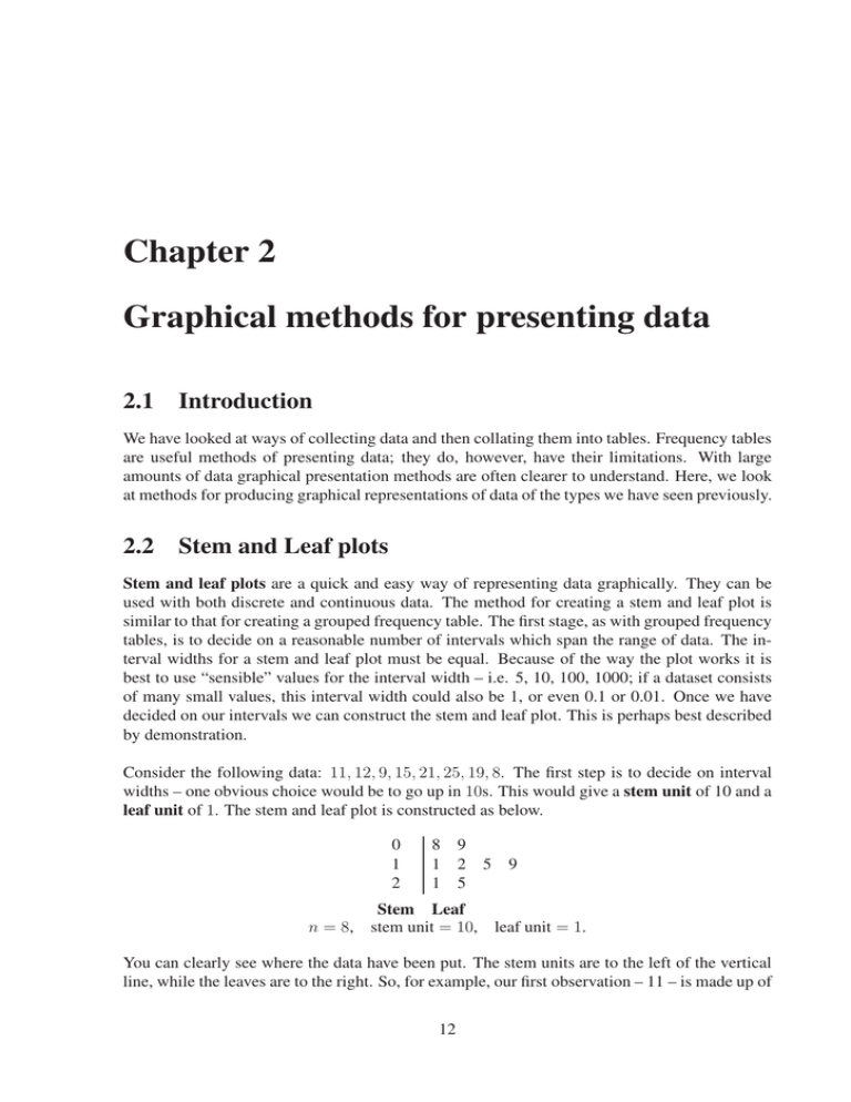
Chapter 2
Graphical methods for presenting data
2.1 Introduction
We have looked at ways of collecting data and then collating them into tables. Frequency tables
are useful methods of presenting data; they do, however, have their limitations. With large
amounts of data graphical presentation methods are often clearer to understand. Here, we look
at methods for producing graphical representations of data of the types we have seen previously.
2.2 Stem and Leaf plots
Stem and leaf plots are a quick and easy way of representing data graphically. They can be
used with both discrete and continuous data. The method for creating a stem and leaf plot is
similar to that for creating a grouped frequency table. The first stage, as with grouped frequency
tables, is to decide on a reasonable number of intervals which span the range of data. The interval widths for a stem and leaf plot must be equal. Because of the way the plot works it is
best to use “sensible” values for the interval width – i.e. 5, 10, 100, 1000; if a dataset consists
of many small values, this interval width could also be 1, or even 0.1 or 0.01. Once we have
decided on our intervals we can construct the stem and leaf plot. This is perhaps best described
by demonstration.
Consider the following data: 11, 12, 9, 15, 21, 25, 19, 8. The first step is to decide on interval
widths – one obvious choice would be to go up in 10s. This would give a stem unit of 10 and a
leaf unit of 1. The stem and leaf plot is constructed as below.
0
1
2
8 9
1 2 5
1 5
9
Stem Leaf
n = 8, stem unit = 10, leaf unit = 1.
You can clearly see where the data have been put. The stem units are to the left of the vertical
line, while the leaves are to the right. So, for example, our first observation – 11 – is made up of
12
CHAPTER 2. GRAPHICAL METHODS FOR PRESENTING DATA
13
a stem unit of one 10 and a leaf unit one 1. It is important to give an equal amount of space to
each leaf value – by doing so, we can get a clear picture of any patterns in the data (it’s almost
like a bar–chart on its side – but it still shows the “raw” observations!). Before producing a stem
and leaf plot, it will probably help to first write down the data in ascending numerical order.
Example 1: Percentage returns on a share
As you might imagine, the interval width does not have to be 10. The following numbers show
the percentage returns on an ordinary share for 23 consecutive months:
–0.2 –2.1 1.0 0.1
1.7 –1.3 –1.2 0.9
–0.5 2.4 –2.3 1.5 1.2 –0.6 2.4 –1.2
0.5 0.1 –0.1 0.3 –0.4 0.5 0.9
Here, the largest value is 2.4 and the smallest –2.3, and we have lots of decimal values in
between. Thus, it seems sensible here to have a stem unit of 1 and a leaf unit of 0.1. A stem and
leaf diagram for this set of returns then might look like:
–2
–1
–0
0
1
2
1
2
2
1
0
4
3
3
5
9
5
4
2
6
5
2
1 4
1 3
7
5 9
Stem Leaf
n = 23, stem unit = 1, leaf unit = 0.1.
Example 2: Unemployment rates in the U.S.
Hopefully, that should all seem fine so far. So what can go wrong? Consider the following data,
which are the percentage unemployment rates for 10 U.S. states:
17
18 15 14 12
19 20 21 24
15
If you were to choose 10 as the interval width (i.e. go up in 10s), the stem and leaf plot would
look like
1
2
2
0
4 5
1 4
5 7 8
9
Stem Leaf
n = 10, stem unit = 10, leaf unit = 1.
Here, the interval width is too large, resulting in only two intervals for our data. With such few
intervals it is difficult to identify any patterns in the data. We can get a better idea about what is
going on if we choose a smaller interval width – say 5. Doing so gives the following stem and
leaf plot:
CHAPTER 2. GRAPHICAL METHODS FOR PRESENTING DATA
1
1
2
2 4
5 5
0 1
14
7 8 9
4
Stem Leaf
n = 10, stem unit = 10, leaf unit = 1.
Notice now that there are two 1s in the stem – one for observations between 10 and 14 (inclusive)
and another for observations between 15 and 19 (inclusive). Thus, the stem unit is still 10, but
the interval width is now only 5. Changing the interval width like this produces a plot which
starts to show some sort of pattern in the data – indeed, this is the intention of such graphical
presentations. We could, however, go to the other extreme and have too many intervals. If
this were the case, any pattern would again be lost because lots of intervals would contain no
observations at all. So choose your interval width carefully!
Example 3: Call centre data
Let’s work through the following example. The observations in the table below are the recorded
time it takes to get through to an operator at a telephone call centre (in seconds).
54
45
30
Stem
n=
56 50 67 55
51 47 53 29
39 65 54 44
38 49 45 39
42 44 61 51
54 72 65 58
50
50
62
Leaf
stem unit =
leaf unit =
CHAPTER 2. GRAPHICAL METHODS FOR PRESENTING DATA
15
Example 4: Production line data
If there is more than one significant figure in the data, the extra digits are cut (or truncated), not
rounded, to the nearest value; that is to say, 2.97 would become 2.9, not 3.0. To illustrate this,
consider the following data on lengths of items on a production line (in cm):
2.97 3.81 2.54 2.01 3.49 3.09 1.99 2.64 2.31 2.22
The stem and leaf plot for this is as follows:
1
2
2
3
3
9
0
5
0
8
2 3
6 9
4
n = 10,
stem unit = 1 cm, leaf unit = 0.1 cm.
Here the interval width is 0.5. This allows for greater clarity in the plot. Why do you think we
cut the extra digits?
Example 5: student marks
The stem and leaf plot below represents the marks on a test for 50 students.
1
1
2
3
4
5
4
5
0
2
0
0
7
0
3
0
0
n = 50,
7
1
3
1
0
9
1
3
2
9
1 2
4 5
2 3
2 4 4
5 6 7
3 4 4
4 5
7 8
5
7 7
8 9
8 8 8
9 9
stem unit = 10, leaf unit = 1.
It’s easy to see some of the advantages of graphically presenting data. For example, here you
can clearly see that the data are centred around a value in the low 30’s and fall away on either
side. From stem and leaf plots we can quickly and easily tell if the distribution of the data
is symmetric or asymmetric. We can see whether there are any outliers, that is, observations
which are either much larger or much smaller than is typical of the data. We could perhaps even
tell whether the data are multi–modal, that is to say, whether there are two or more peaks on
the graph with a gap between them. If so, this could suggest that the sample contains data from
two or more groups.
CHAPTER 2. GRAPHICAL METHODS FOR PRESENTING DATA
16
2.2.1 Using Minitab
With the small data sets we have seen so far, it is obviously relatively easy to create stem and
leaf plots by hand. With larger data sets this would be more problematic and certainly more
time consuming. Fortunately, there are computer packages that will create these plots for us –
Minitab is one such package, and can be found on most university computers.
Details and guidance on using Minitab will be provided in the computer practical sessions in
week 7.
2.3 Bar Charts
Bar charts are a commonly–used and clear way of presenting categorical data or any ungrouped
discrete frequency observations.
For example, recall the example on students’ modes of transport:
Student
1
2
3
4
5
6
7
8
9
10
Mode
Car
Walk
Car
Walk
Bus
Metro
Car
Bike
Walk
Car
Student
11
12
13
14
15
16
17
18
19
20
Mode
Walk
Walk
Metro
Bus
Train
Bike
Bus
Bike
Bike
Metro
Student
21
22
23
24
25
26
27
28
29
30
The first logical step is to put these into a frequency table, giving
Mode Frequency
Car
10
Walk
7
Bike
4
Bus
4
Metro
4
Train
1
Total
30
Mode
Walk
Metro
Car
Car
Car
Bus
Car
Walk
Car
Car
CHAPTER 2. GRAPHICAL METHODS FOR PRESENTING DATA
17
We can then present this information as a bar chart, by following the five step process shown
below:
1. First decide what goes on each axis of the chart. By convention the variable being measured goes on the horizontal (x–axis) and the frequency goes on the vertical (y–axis).
2. Next decide on a numeric scale for the frequency axis. This axis represents the frequency
in each category by its height. It must start at zero and include the largest frequency. It is
common to extend the axis slightly above the largest value so you are not drawing to the
edge of the graph.
3. Having decided on a range for the frequency axis we need to decide on a suitable number
scale to label this axis. This should have sensible values, for example, 0, 1, 2, . . . , or
0, 10, 20 . . . , or other such values as make sense given the data.
4. Draw the axes and label them appropriately.
5. Draw a bar for each category. When drawing the bars it is essential to ensure the following:
– the width of each bar is the same;
– the bars are separated from each other by equally sized gaps.
This gives the following bar chart:
10
8
Frequency
6
4
2
Car
Walk
Bike
Bus
Metro
Train
This bar chart clearly shows that the most popular mode of transport is the car and that the
metro, bus and cycling are all equally popular (in our small sample). Bar charts provide a
simple method of quickly spotting simple patterns of popularity within a discrete data set.
CHAPTER 2. GRAPHICAL METHODS FOR PRESENTING DATA
18
2.4 Histograms
Bar charts have their limitations; for example, they cannot be used to present continuous data.
When dealing with continuous random variables a different kind of graph is required. This is
called a histogram. At first sight these look similar to bar charts. There are, however, two
critical differences:
• the horizontal (x-axis) is a continuous scale. As a result of this there are no gaps between
the bars (unless there are no observations within a class interval);
• the height of the rectangle is only proportional to the frequency if the class intervals are
all equal. With histograms it is the area of the rectangle that is proportional to their
frequency.
Initially we will only consider histograms with equal class intervals. Those with uneven class
intervals require more careful thought.
Producing a histogram is much like producing a bar chart and in many respects can be considered to be the next stage after producing a grouped frequency table. In reality, it is often best
to produce a frequency table first which collects all the data together in an ordered format. Once
we have the frequency table, the process is very similar to drawing a bar chart.
1. Find the maximum frequency and draw the vertical (y–axis) from zero to this value,
including a sensible numeric scale.
2. The range of the horizontal (x–axis) needs to include not only the full range of observations but also the full range of the class intervals from the frequency table.
3. Draw a bar for each group in your frequency table. These should be the same width and
touch each other (unless there are no data in one particular class).
The frequency table for the data on service times for a telephone call centre (Section 1.3.2) was
Service time
Frequency
175 ≤ time < 180
1
180 ≤ time < 185
3
185 ≤ time < 190
3
190 ≤ time < 195
6
195 ≤ time < 200
10
200 ≤ time < 205
12
205 ≤ time < 210
8
210 ≤ time < 215
3
215 ≤ time < 220
3
220 ≤ time < 225
1
Total
50
CHAPTER 2. GRAPHICAL METHODS FOR PRESENTING DATA
19
The histogram for these data is:
12
10
Frequency
8
6
4
2
175
180
185
190
195
200
205
210
215
220
225
Time (s)
Histograms are useful tools in data analysis. They are easy to produce in Minitab for large
data sets and provide a clear visual representation of the data. Using histograms, it is easy
to spot the modal or most popular class in the data, i.e. the one with the highest peak. It
is also easy to spot simple patterns in the data. Is the frequency distribution symmetric, as
the histograms produced above, or is it skewed to one side like the left–hand histogram in the
following graphic?
CHAPTER 2. GRAPHICAL METHODS FOR PRESENTING DATA
20
Histograms also allow us to make early judgements as to whether all our data come from the
same population. Consider the right–hand histogram in the graphic above. It clearly contains
two separate modes (peaks), each of which has its own symmetric pattern of data. This clearly
suggests that the data come from two separate populations, one centred around 85 with a narrow
spread and one centred around 100 with a wider spread. In real situations it is unlikely that the
difference would be as dramatic, unless you had a poor sampling method. However, the drawing
of histograms is often the first stage of a more complex analysis.
Finally, when drawing histograms be aware of observations on variables which have boundaries
on their ranges. For example heights, weights, times to complete tasks etc. can not take negative
values so there is a lower limit at zero. Computer programs do not automatically know this. You
should make sure that the lower limit of the first class interval is not negative in such cases.
We have seen some basic ways in which we might present data graphically. These methods
will often provide the mainstay of business presentations. There are, however, other techniques
which are useful and offer advantages in some applications over histograms and bar charts.
CHAPTER 2. GRAPHICAL METHODS FOR PRESENTING DATA
21
2.5 Percentage Relative Frequency Histograms
When we produced frequency tables in Section 1.3, we included a column for percentage relative frequency. This contained values for the frequency of each group, relative to the overall
sample size, expressed as a percentage. For example, a percentage relative frequency table for
the data on service time (in seconds) for calls to a credit card service centre is:
Service time
Frequency
175 ≤ time < 180
1
180 ≤ time < 185
3
185 ≤ time < 190
3
190 ≤ time < 195
6
195 ≤ time < 200
10
200 ≤ time < 205
12
205 ≤ time < 210
8
210 ≤ time < 215
3
215 ≤ time < 220
3
220 ≤ time < 225
1
Totals
50
Relative Frequency (%)
2
6
6
12
20
24
16
6
6
2
100
You can plot these data like an ordinary histogram, or, instead of using frequency on the vertical
axis (y-axis), you could use the percentage relative frequency.
24
20
Relative
frequency
(%)
16
12
8
4
175
180
185
190
195
200
205
210
215
220
225
Time (s)
Note that the y-axis now contains the relative percentages rather than the frequencies. You
might well ask “why would we want to do this?”.
CHAPTER 2. GRAPHICAL METHODS FOR PRESENTING DATA
22
These percentage relative frequency histograms are useful when comparing two samples that
have different numbers of observations. If one sample were larger than the other then a frequency histogram would show a difference simply because of the larger number of observations.
Looking at percentages removes this difference and enables us to look at relative differences.
For example, in the following graph there are data from two groups and four times as many
data points for one group as the other. The left-hand plot shows an ordinary histogram and it
is clear that the comparison between groups is masked by the quite different sample sizes. The
right-hand plot shows a histogram based on (percentage) relative frequencies and this enables a
much more direct comparison of the distributions in the two groups.
Overlaying histograms on the same graph can sometimes not produce such a clear picture,
particularly if the values in both groups are close or overlap one another significantly.
CHAPTER 2. GRAPHICAL METHODS FOR PRESENTING DATA
23
2.6 Relative Frequency Polygons
These are a natural extension of the relative frequency histogram. They differ in that, rather than
drawing bars, each class is represented by one point and these are joined together by straight
lines. The method is similar to that for producing a histogram:
1. Produce a percentage relative frequency table.
2. Draw the axes
– The x-axis needs to contain the full range of the classes used.
– The y-axis needs to range from 0 to the maximum percentage relative frequency.
3. Plot points: pick the mid point of the class interval on the x-axis and go up until you reach
the appropriate percentage value on the y-axis and mark the point. Do this for each class.
4. Join adjacent points together with straight lines.
The relative frequency polygon is exactly the same as the relative frequency histogram, but
instead of having bars we join the mid–points of the top of each bar with a straight line. Consider
the following simple example.
Class Interval
0 ≤ x < 10
10 ≤ x < 20
20 ≤ x < 30
30 ≤ x < 40
40 ≤ x < 50
Mid Point % Relative Frequency
5
10
15
20
25
35
35
25
45
10
This can be easily drawn by hand:
Relative frequency polygon
Relative 40
frequency
(%)
30
20
10
0
10
0
20
30
40
50
x
CHAPTER 2. GRAPHICAL METHODS FOR PRESENTING DATA
24
These percentage relative frequency polygons are very useful for comparing two or more samples – we can easily “overlay” many relative frequency polygons, but overlaying the corresponding histograms could get really messy! Consider the following data on gross weekly income
(in £) collected from two sites in Newcastle. Let us suppose that many more responses were
collected in Jesmond so that a direct comparison of the frequencies using a standard histogram
is not appropriate. Instead we use relative frequencies.
Weekly Income (£)
West Road (%)
0 ≤ income < 100
9.3
100 ≤ income < 200
26.2
200 ≤ income < 300
21.3
300 ≤ income < 400
17.3
400 ≤ income < 500
11.3
500 ≤ income < 600
6.0
600 ≤ income < 700
4.0
700 ≤ income < 800
3.3
800 ≤ income < 900
1.3
900 ≤ income < 1000
0.0
Jesmond Road (%)
0.0
0.0
4.5
16.0
29.7
22.9
17.7
4.6
2.3
2.3
Minitab was used to produce the following plot of the percentage relative frequancy polygons
for the two groups.
We can clearly see the differences between the two samples. The line connecting the boxes
represents the data from West Road and the line connecting the circles represents those for
Jesmond Road. The distribution of incomes on West Road is skewed towards lower values,
whilst those on Jesmond Road are more symmetric. The graph clearly shows that income in the
Jesmond Road area is higher than that in the West Road area.
CHAPTER 2. GRAPHICAL METHODS FOR PRESENTING DATA
25
2.7 Cumulative Frequency Polygons (Ogive)
Cumulative percentage relative frequency is also a useful tool. The cumulative percentage relative frequency is simply the sum of the percentage relative frequencies at the end of each
class interval (i.e. we add the frequencies up as we go along). Consider the example from the
previous section:
Class Interval
0 ≤ x < 10
10 ≤ x < 20
20 ≤ x < 30
30 ≤ x < 40
40 ≤ x < 50
% Relative Frequency
10
20
35
25
10
Cumulative % Relative Frequency
10
30
65
90
100
At the upper limit of the first class the cumulative % relative frequency is simply the % relative
frequency in the first class, i.e. 10. However, at the end of the second class, at 20, the cumulative
% relative frequency is 10 + 20 = 30. The cumulative % relative frequency at the end of the
last class must be 100.
The corresponding graph, or ogive, is simple to produce by hand:
1. Draw the axes.
2. Label the x-axis with the full range of the data and the y-axis from 0 to 100%.
3. Plot the cumulative % relative frequency at the end point of each class.
4. Join adjacent points, starting at 0% at the lowest class boundary.
Ogive
100
80
Cumulative
relative 60
frequency
(%)
40
20
0
10
0
20
30
40
50
x
CHAPTER 2. GRAPHICAL METHODS FOR PRESENTING DATA
26
For example, Minitab was used to produce the ogive below for the income data from the West
Road survey:
This graph instantly tells you many things. To see what percentage of respondents earn less
than £x per week:
1. Find x on the x-axis and draw a line up from this value until you reach the ogive;
2. From this point trace across to the y-axis;
3. Read the percentage from the y-axis.
If we wanted to know what percentage of respondents in the survey in West Road earn less than
£250 per week, we simply find £250 on the x-axis, trace up to the ogive and then trace across
to the y-axis and we can read a figure of about 47%. The process obviously works in reverse.
If we wanted to know what level of income 50% of respondents earned, we would trace across
from 50% to the ogive and then down to the x-axis and read a value of about £300.
CHAPTER 2. GRAPHICAL METHODS FOR PRESENTING DATA
27
Ogives can also be used for comparison purposes. The following plot contains the ogives for
the income data at both the West Road and Jesmond Road sites.
It clearly shows the ogive for Jesmond Road is shifted to the right of that for West Road. This
tells us that the surveyed incomes are higher on Jesmond Road. We can compare the percentages of people earning different income levels between the two sites quickly and easily.
This technique can also be used to great effect for examining the changes before and after
the introduction of a marketing strategy. For example, daily sales figures of a product for a
period before and after an advertising campaign might be plotted. Here, a comparison of the
two ogives can be used to help assess whether or not the campaign has been successful.
CHAPTER 2. GRAPHICAL METHODS FOR PRESENTING DATA
28
2.8 Other graphical summaries
2.8.1 Multiple Bar Charts
The data below gives the daily sales of CDs (in £) by music type for an independent retailer.
Day
Monday
Tuesday
Wednesday
Thursday
Friday
Saturday
Sunday
Total
Chart Dance Rest
Total
12000 10000 2700 24700
11000
8000 3000 22000
9000
6000 2000 17000
10000
5000 2500 17500
12000 11000 3000 26000
19000 12000 4000 35000
10000
8000 2000 20000
83000 60000 19200 162200
Bar charts could be drawn of total sales per music type in the week, or of total daily sales. It
might be interesting to see daily sales broken down into music types. This can be done in a
similar manner to the bar charts produced previously. The only difference is that the height of
the bars is dictated by the total daily sales, and each bar has segments representing each music
type.
The Minitab worksheet and chart this produces are shown below:
These types of charts are particularly good for presenting such financial information or illustrating any breakdown of data over time – for example, the number of new cars sold by month
and model.
CHAPTER 2. GRAPHICAL METHODS FOR PRESENTING DATA
29
2.8.2 Pie charts
Pie charts are simple diagrams for displaying categorical or grouped data. These charts are
commonly used within industry to communicate simple ideas, for example market share. They
are used to show the proportions of a whole. They are best used when there are only a handful
of categories to display.
A pie chart consists of a circle divided into segments, one segment for each category. The
size of each segment is determined by the frequency of the category and measured by the angle
of the segment. As the total number of degrees in a circle is 360, the angle given to a segment
is 360◦ times the fraction of the data in the category, that is
angle =
Number in category
× 360.
Total number in sample (n)
Consider the data on newspaper sales to 650 students.
Paper
Frequency Degrees
The Times
140
77.5
The Sun
200
110.8
The Sport
50
27.7
The Guardian
120
66.5
The Financial Times
20
11.1
The Mirror
80
44.3
The Daily Mail
10
5.5
The Independent
30
16.6
Totals
650
360.0
The pie chart is constructed by first drawing a circle and then dividing it up into segments whose
angles are calculated using this formula.
Minitab was used to produce the following pie chart:
CHAPTER 2. GRAPHICAL METHODS FOR PRESENTING DATA
30
It shows that The Sun, The Times and The Guardian are the most popular papers.
Note that the pie chart is a simple circle. Some computer software will draw “perspective”
pie charts, pie charts with slices detached etc. It is best to avoid such gimmicks which merely
obscure the information contained in the chart.
2.8.3 Scatter Plots
Scatter plots are used to plot two variables which you believe might be related, for example,
height and weight, advertising expenditure and sales, or age of machinery and maintenance
costs.
Consider the following data for monthly output and total costs at a factory.
Total costs (£)
10300
12000
12000
13500
12200
14200
10800
18200
16200
19500
17100
19200
Monthly Output
2400
3900
3100
4500
4100
5400
1100
7800
7200
9500
6400
8300
If you were interested in the relationship between the cost of production and the number of units
produced you could easily plot this by hand.
1. The “response” variable is placed on the y-axis. Here we are trying to understand how
total costs relate to monthly output and so the response variable is “total costs”.
2. The variable that is used to try to explain the response variable (here, monthly output) is
placed on the x-axis.
3. Plot the pairs of points on the graph.
This graph can be produced using Minitab (Select Graph then Scatterplot then Simple
and insert the required variables).
CHAPTER 2. GRAPHICAL METHODS FOR PRESENTING DATA
31
The plot highlights a clear relationship between the two variables: the more units made, the
more it costs in total. This relationship is shown on the graph by the upwards trend within the
data – as monthly output increases so too does total cost. A downwards sloping trend would
imply that as output increased, total costs declined, an unlikely scenario. This type of plot is the
first stage of a more sophisticated analysis which we will develop in Semester 2 of this course.
CHAPTER 2. GRAPHICAL METHODS FOR PRESENTING DATA
32
2.8.4 Time Series Plots
So far we have only considered data where we can (at least for some purposes) ignore the order
in which the data come. Not all data are like this. One exception is the case of time series
data, that is, data collected over time. Examples include monthly sales of a product, the price
of a share at the end of each day or the air temperature at midday each day. Such data can be
plotted by using a scatter plot, but with time as the (horizontal) x-axis, and where the points
are connected by lines.
Consider the following data (overleaf) on the number of computers sold (in thousands) by
quarter (January-March, April-June, July-September, October-December) at a large warehouse
outlet.
Quarter
Q1 2000
Q2 2000
Q3 2000
Q4 2000
Q1 2001
Q2 2001
Q3 2001
Q4 2001
Q1 2002
Q2 2002
Q3 2002
Q4 2002
Q1 2003
Q2 2003
Q3 2003
Q4 2003
Q1 2004
Q2 2004
Q3 2004
Units Sold
86.7
94.9
94.2
106.5
105.9
102.4
103.1
115.2
113.7
108.0
113.5
132.9
126.3
119.4
128.9
142.3
136.4
124.6
127.9
By hand, a time series plot is constructed as follows:
1. Draw the x-axis and label over the time scale.
2. Draw the y-axis and label with an appropriate scale.
3. Plot each point according to time and value.
4. Draw lines connecting all points.
CHAPTER 2. GRAPHICAL METHODS FOR PRESENTING DATA
33
The time series plot is:
The plot clearly shows us two things: firstly, that there is an upwards trend to the data, and
secondly that there is some regular variation around this trend. We will come back to more
sophisticated techniques for analysing time series data later in the course.
CHAPTER 2. GRAPHICAL METHODS FOR PRESENTING DATA
34
2.9 Exercises
1. The following table shows the weight (in kilograms) of 50 sacks of potatoes leaving a
farm shop.
10.41
11.24
9.36
11.36
10.05
9.91
8.70
9.27
10.61
10.72
10.06
10.58
9.63
10.82
11.30
10.26
9.49
11.69
8.83
10.63
9.38
8.55
10.33
8.93
11.01
10.67
10.98
9.66
10.11
12.86
11.36
10.47
10.05
10.08
9.72
10.21
10.01
9.52
10.37
10.62
9.65
8.22
11.57
9.53
10.67
8.18
9.92
10.40
9.73
10.26
Display these data in a stem and leaf plot. Note the number of decimal places and adjust
accordingly. State clearly both the stem and the leaf units.
2. A market researcher asked 650 students what their favourite daily newspaper was. The results are summarised in the frequency table below. Represent these data in an appropriate
graphical manner.
The Times
140
The Sun
200
The Sport
50
The Guardian
120
The Financial Times 20
The Mirror
80
The Daily Mail
10
The Independent
30
3. Produce a histogram for the data on length of mobile phone calls from the exercises in
Chapter 1 (listed again below) and comment on it.
281.4
312.7
270.7
304.1
305.4
278.3
293.2
299.6
281.1
314.8
293.4
327.7
293.9
320.7
317.9
300.1
267.5
293.9
306.9
292.0
306.5
311.5
310.9
283.6
289.5
292.6
326.9
303.9
310.2
302.4
286.6
314.8
346.4
337.5
286.9
312.9
257.7
323.7
301.6
267.9
298.4
303.3
304.6
259.6
300.5
302.5
285.9
263.5
313.9
292.0
CHAPTER 2. GRAPHICAL METHODS FOR PRESENTING DATA
35
4. Consider the following data for daily sales at a small record shop, before and after a local
radio advertising campaign.
Daily Sales
Before
1000 ≤ sales < 2000
10
2000 ≤ sales < 3000
30
3000 ≤ sales < 4000
40
4000 ≤ sales < 5000
20
5000 ≤ sales < 6000
15
6000 ≤ sales < 7000
12
7000 ≤ sales < 8000
10
8000 ≤ sales < 9000
8
9000 ≤ sales < 10000
0
Totals
145
After
7
10
25
35
37
40
20
10
5
189
(a) Calculate the percentage relative frequency for before and after.
(b) Calculate the cumulative percentage relative frequency for before and after.
(c) Plot the relative frequency polygons for both on one graph and comment.
(d) Plot the ogives for both on one graph.
(e) Find the level of sales, before and after, that are reached on 25%, 50% and 75% of
days.