Section 13
Kolmogorov-Smirnov test.
Suppose that we have an i.i.d. sample X1 , . . . , Xn with some unknown distribution P and we
would like to test the hypothesis that P is equal to a particular distribution P0 , i.e. decide
between the following hypotheses:
H0 : P = P 0 , H 1 : P =
⇒ P0 .
We already know how to test this hypothesis using chi-squared goodness-of-fit test. If dis­
tribution P0 is continuous we had to group the data and consider a weaker discretized null
hypothesis. We will now consider a different test for H0 based on a very different idea that
avoids this discretization.
1
1
0.9
0.9
all data
normal fit
0.8
0.7
Cumulative probability
Cumulative probability
0.8
0.6
0.5
0.4
0.3
0.7
0.6
0.5
0.4
0.3
0.2
0.2
0.1
0.1
0
96
96.5
97
97.5
men data
’men’ fit
women data
’women’ fit
98
98.5
Data
99
99.5
100
0
100.5
96.5
97
97.5
98
98.5
Data
99
99.5
100
100.5
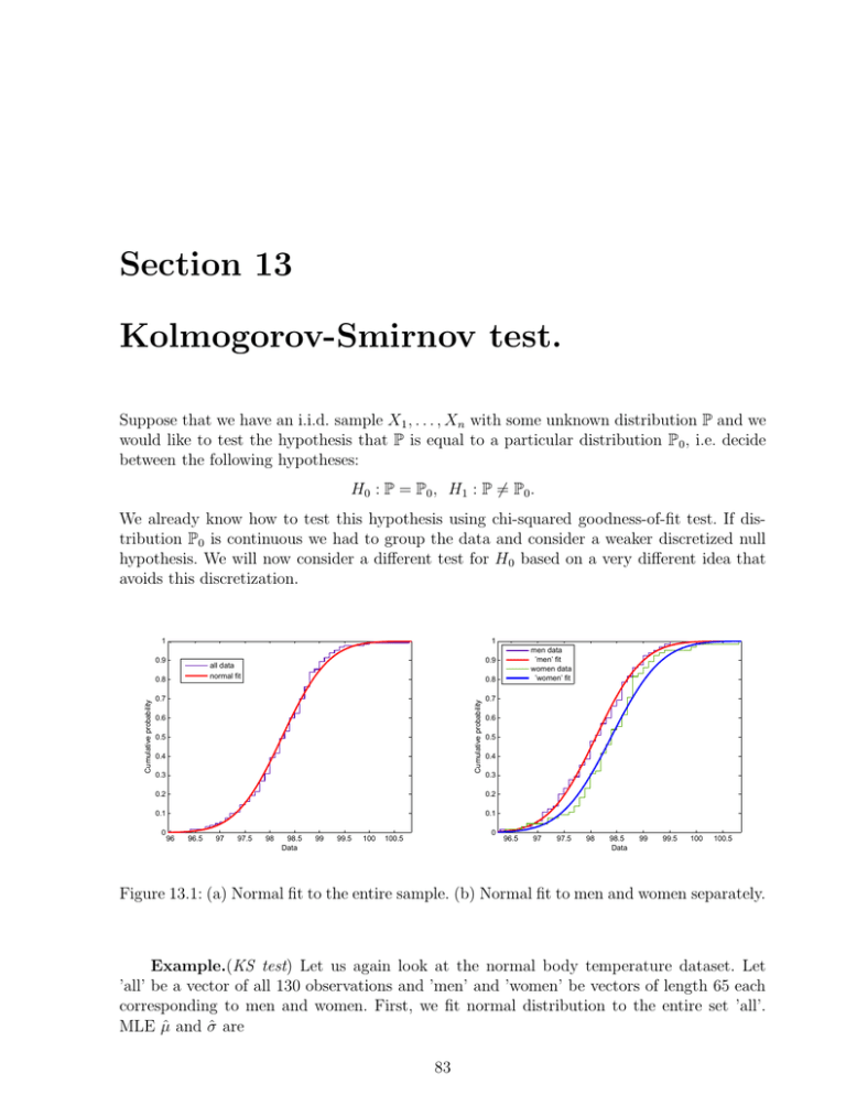
Figure 13.1: (a) Normal fit to the entire sample. (b) Normal fit to men and women separately.
Example.(KS test) Let us again look at the normal body temperature dataset. Let
’all’ be a vector of all 130 observations and ’men’ and ’women’ be vectors of length 65 each
corresponding to men and women. First, we fit normal distribution to the entire set ’all’.
MLE µ̂ and �
ˆ are
83
mean(all) = 98.2492, std(all,1) = 0.7304.
We see in figure 13.1 (a) that this distribution fits the data very well. Let us perfom KS test
that the data comes from this distribution N (µ̂, �
ˆ 2 ). To run the test, first, we have to create
2
a vector of N(µ̂, �
ˆ ) c.d.f. values on the sample ’all’ (it is a required input in Matlab KS test
function):
CDFall=normcdf(all,mean(all),std(all,1));
Then we run Matlab ’kstest’ function
[H,P,KSSTAT,CV] = kstest(all,[all,CDFall],0.05)
which outputs
H = 0, P = 0.6502, KSSTAT = 0.0639, CV = 0.1178.
We accept H0 since the p-value is 0.6502. ’CV’ is a critical value such that H0 is rejected if
statistic ’KSSTAT’>’CV’.
Remark. KS test is designed to test a simple hypothesis P = P0 for a given specified
distribution P0 . In the example above we estimated this distribution, N(µ̂, �
ˆ 2 ) from the data
so, formally, KS is inaccurate in this case. There is a version of KS test, called Lilliefors
test, that tests normality of the distribution by comparing the data with a fitted normal
distribution as we did above, but with a correction to give a more accurate approximation
of the distribution of the test statistic.
Example. (Lilliefors test.) We use Matlab function
[H,P,LSTAT,CV] = lillietest(all)
that outputs
H = 0, P = 0.1969, LSTAT = 0.0647, CV = 0.0777.
We accept the normality of ’all’ with p-value 0.1969.
Example. (KS test for two samples.) Next, we fit normal distributions to ’men’ and
’women’ separately, see figure 13.1 (b). We see that they are slightly different so it is a natural
question to ask whether this difference is statistically significant. We already looked at this
problem in the lecture on t-tests. Under a reasonable assumption that body temperatures
of men and women are normally distributed, all t-tests - paired, with equal variances and
with unequal variances - rejected the hypothesis that the mean body temperatures are equal
µmen = µwomen . In this section we will describe a KS test for two samples that tests the
hypothesis H0 : P1 = P2 that two samples come from the same distribution. Matlab function
’kstest2’
[H,P,KSSTAT] = kstest2(men, women)
84
outputs
H = 0, P =
0.1954, KSSTAT = 0.1846.
It accepts the null hypothesis since p-value 0.1954 > 0.05 = � - a default value of the level
of significance. According to this test, the difference between two samples is not significant
enough to say that they have different distribution.
Let us now explain some ideas behind these tests. Let us denote by F (x) = P(X1 � x)
a c.d.f. of a true underlying distribution of the data. We define an empirical c.d.f. by
n
1
�
Fn (x) = Pn (X � x) =
I(Xi � x)
n i=1
that counts the proportion of the sample points below level x. For any fixed point x ∞ R the
law of large numbers implies that
n
1 �
Fn (x) =
I(Xi � x) � EI(X1 � x) = P(X1 � x) = F (x),
n i=1
i.e. the proportion of the sample in the set (−→, x] approximates the probability of this set.
It is easy to show from here that this approximation holds uniformly over all x ∞ R:
sup |Fn (x) − F (x)| � 0
x�R
i.e. the largest difference between Fn and F goes to 0 in probability. The key observation in
the Kolmogorov-Smirnov test is that the distribution of this supremum does not depend on
the ’unknown’ distribution P of the sample, if P is continuous distribution.
Theorem 1. If F (x) is continuous then the distribution of
sup |Fn (x) − F (x)|
x�R
does not depend on F .
Proof. Let us define the inverse of F by
F −1 (y) = min{x : F (x) ≈ y}.
Then making the change of variables y = F (x) or x = F −1 (y) we can write
P(sup |Fn (x) − F (x)| � t) = P( sup |Fn (F −1 (y)) − y| � t).
0�y�1
x�R
Using the definition of the empirical c.d.f. Fn we can write
n
Fn (F
−1
n
1
�
1
�
I(Xi � F −1 (y)) =
I(F (Xi ) � y)
(y)) =
n
i=1
n
i=1
85
1
0.9
0.8
sup |Fn (x) − F (x)|
Cumulative probability
0.7
x
0.6
0.5
0.4
0.3
0.2
0.1
Sfrag replacements
0
96.5
97
97.5
98
98.5
99
99.5
100
100.5
Figure 13.2: Kolmogorov-Smirnov test statistic.
and, therefore,
n
�
� 1
�
�
�
�
�
P( sup |Fn (F −1 (y)) − y| � t) = P sup
�
I(F (Xi ) � y) − y �
� t
.
0�y�1
0�y�1 n
i=1
The distribution of F (Xi ) is uniform on the interval [0, 1] because the c.d.f. of F (X1 ) is
P(F (X1 ) � t) = P(X1 � F −1 (t)) = F (F −1 (t)) = t.
Therefore, the random variables
Ui = F (Xi ) for i � n
are independent and have uniform distribution on [0, 1], so we proved that
n
�
� 1
�
�
�
�
P(sup |Fn (x) − F (x)| � t) = P sup
�
I(Ui � y) − y �
� t
0�y�1 n
x�R
i=1
�
which is clearly independent of F .
86
To motivate KS test, we will need one more result which we will formulate without
proof. First of all, let us note that for a fixed point x the CLT implies that
�
�
≥
d
n(Fn (x) − F (x)) � N 0, F (x)(1 − F (x))
because F (x)(1 − F (x)) is the variance of I(X1 � x). If turns out that if we consider
≥
n sup |Fn (x) − F (x)|
x�R
it will also converge in distribution.
Theorem 2. We have,
P
�≥
�
n sup |Fn (x) − F (x)| � t � H(t) = 1 − 2
x�R
�
�
(−1)i−1 e−2i
2t
i=1
where H(t) is the c.d.f. of Kolmogorov-Smirnov distribution.
Let us reformulate the hypotheses in terms of cumulative distribution functions:
H0 : F = F0 vs. H1 : F ⇒= F0 ,
where F0 is the c.d.f. of P0 . Let us consider the following statistic
≥
Dn = n sup |Fn (x) − F0 (x)|.
x�R
If the null hypothesis is true then, by Theorem 1, we distribution of Dn can be tabulated
(it will depend only on n). Moreover, if n is large enough then the distribution of Dn is
approximated by Kolmogorov-Smirnov distribution from Theorem 2. On the other hand,
suppose that the null hypothesis fails, i.e. F =
⇒ F0 . Since F is the true c.d.f. of the data, by
law of large numbers the empirical c.d.f. Fn will converge to F and as a result it will not
approximate F0 , i.e. for large n we will have
sup |Fn (x) − F0 (x)| > �
x
≥
for some small enough �. Multiplying this by n implies that
≥
≥
Dn = n sup |Fn (x) − F0 (x)| > n�.
x�R
If H0 fails then Dn >
decision rule
≥
n� � +→ as n � →. Therefore, to test H0 we will consider a
�
H0 : D n � c
�=
H1 : D n > c
The threshold c depends on the level of significance � and can be found from the condition
� = P(� =
⇒ H0 |H0 ) = P(Dn ≈ c|H0 ).
87
Since under H0 the distribution of Dn can be tabulated for each n, we can find the threshold
c = c� from the tables. In fact, most statistical table books have these distributions for n up
to 100. Seems like Matlab has these tables built in the ’kstest’ but the distribution of D n
is not available as a separate function. When n is large then we can use KS distribution to
find c since
� = P(Dn ≈ c|H0 ) � 1 − H(c).
and we can use the table for H to find c.
KS test for two samples.
Kolmogorov-Smirnov test for two samples is very similar. Suppose that a first sample
X1 , . . . , Xm of size m has distribution with c.d.f. F (x) and the second ssmple Y1 , . . . , Yn of
size n has distribution with c.d.f. G(x) and we want to test
H0 : F = G vs. H1 : F ⇒= G.
If Fm (x) and Gn (x) are corresponding empirical c.d.f.s then the statistic
Dmn =
� mn �1/2
sup |Fm (x) − Gn (x)|
m+n
x
satisfies Theorems 1 and 2 and the rest is the same
Example. Let us consider a sample of size 10:
0.58, 0.42, 0.52, 0.33, 0.43, 0.23, 0.58, 0.76, 0.53, 0.64
and let us test the hypothesis that the distribution of the sample is uniform on [0, 1] i.e.
H0 : F (x) = F0 (x) = x. The figure 13.3 shows the c.d.f. F0 and empirical c.d.f. Fn (x). To
compute Dn we notice that the largest difference between F0 (x) and Fn (x) is achieved either
before or after one of the jumps, i.e.
�
|Fn (Xi− ) − F (Xi )| - before the ith jump
sup |Fn (x) − F (x)| = max
|Fn (Xi ) − F (Xi )|
- after the ith jump.
1�i�n
0�x�1
Writing these differences for our data we get
before the jump after the jump
|0 − 0.23|
|0.1 − 0.23|
|0.2 − 0.33|
|0.1 − 0.33|
|0.2 − 0.42|
|0.3 − 0.42|
|0.3 − 0.43|
|0.4 − 0.43|
···
The largest value will be achieved at |0.9 − 0.64| = 0.26 and, therefore,
≥
≥
Dn = n sup |Fn (x) − x| = 10 × 0.26 = 0.82.
0�x�1
88
Empirical CDF
1
0.9
0.8
0.7
sup |Fn (x) − x| = 0.26
F(x)
0.6
0�x�1
0.5
0.4
0.3
0.2
0.1
Sfrag replacements
0
0
0.64
0.1
0.2
0.3
0.4
0.5
x
0.6
0.7
0.8
0.9
1
Figure 13.3: Fn and F0 in the example.
If we take the level of significance � = 0.05 and use KS approximation of Theorem 2 to find
threshold c:
1 − H(c) = 0.05 ≤ c = 1.35,
then according to KS test
�=
�
H1 : Dn � 1.35
H2 : Dn > 1.35
we accept the null hypothesis H0 since Dn = 0.82 < c = 1.35.
However, we have only n = 10 observations so the approximation of Theorem 2 might
be inaccurate. We could use the advanced statistical tables to find the distibution of D n for
n = 10 or let Matlab do it. Running
[H,P,KSSTAT,CV] = kstest(X,[X,X],0.05)
(remark1 ) outputs
H = 0, P = 0.4466, KSSTAT = 0.2600, CV = 0.4093.
1
Here the second input of ’kstest’ should be a n × 2 matrix where the first column is the data X and
the second column is the corresponding values of c.d.f. F0 (x). But since we test with F0 (x) = x, the second
column is equal to X and, thus, we input ’[X,X]’
89
≥
Since Matlab function ’kstest’ does not scale the statistic by n since it is using the exact
F (x)| instead of approximation of Theorem 2, the critical value
distribution of supx |F
≥ n (x) −≥
’CV’ mupliplied by n, i.e. 10 × 0.4093 = 1.294 will be exactly our threshold such that
P(Dn > c|H0 ) = � = 0.05.
It is slightly different from c = 1.35 given by the approximation of Theorem 2. So for small
sample sizes it is better to use the exact distribution of Dn .
90