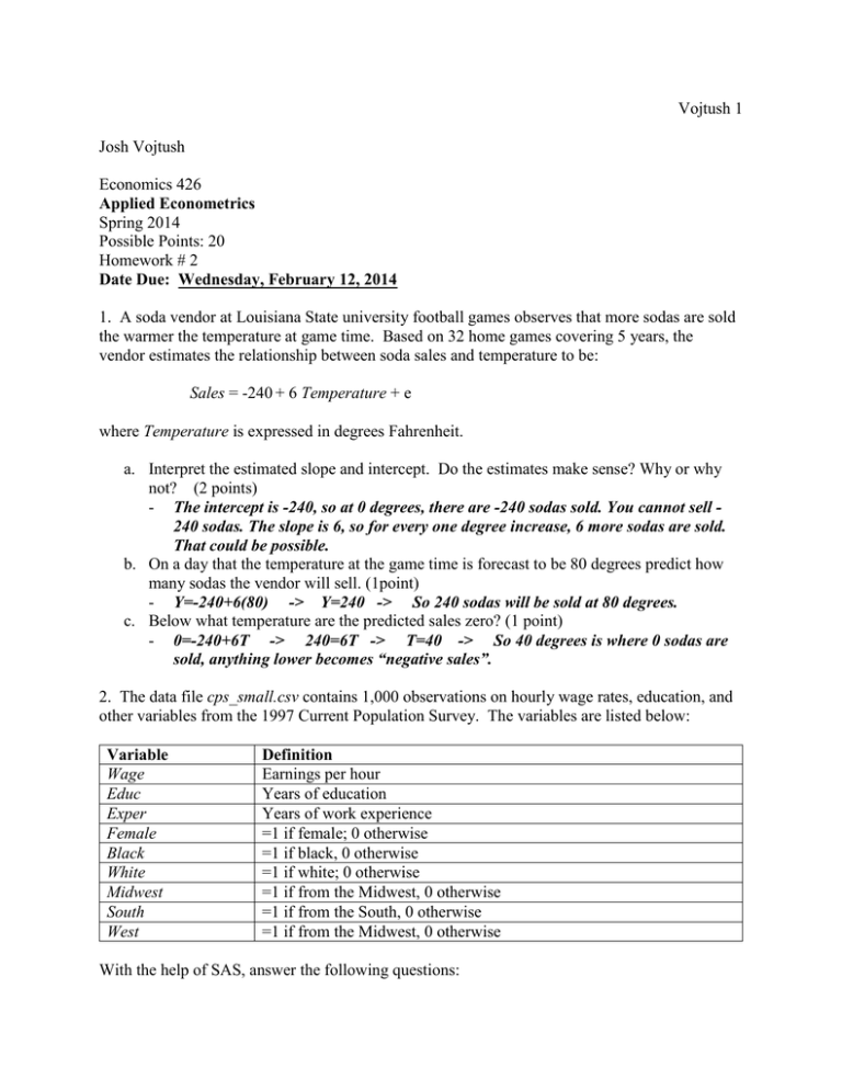
Vojtush 1
Josh Vojtush
Economics 426
Applied Econometrics
Spring 2014
Possible Points: 20
Homework # 2
Date Due: Wednesday, February 12, 2014
1. A soda vendor at Louisiana State university football games observes that more sodas are sold
the warmer the temperature at game time. Based on 32 home games covering 5 years, the
vendor estimates the relationship between soda sales and temperature to be:
Sales = -240 + 6 Temperature + e
where Temperature is expressed in degrees Fahrenheit.
a. Interpret the estimated slope and intercept. Do the estimates make sense? Why or why
not? (2 points)
- The intercept is -240, so at 0 degrees, there are -240 sodas sold. You cannot sell 240 sodas. The slope is 6, so for every one degree increase, 6 more sodas are sold.
That could be possible.
b. On a day that the temperature at the game time is forecast to be 80 degrees predict how
many sodas the vendor will sell. (1point)
- Y=-240+6(80) -> Y=240 -> So 240 sodas will be sold at 80 degrees.
c. Below what temperature are the predicted sales zero? (1 point)
- 0=-240+6T -> 240=6T -> T=40 -> So 40 degrees is where 0 sodas are
sold, anything lower becomes “negative sales”.
2. The data file cps_small.csv contains 1,000 observations on hourly wage rates, education, and
other variables from the 1997 Current Population Survey. The variables are listed below:
Variable
Wage
Educ
Exper
Female
Black
White
Midwest
South
West
Definition
Earnings per hour
Years of education
Years of work experience
=1 if female; 0 otherwise
=1 if black, 0 otherwise
=1 if white; 0 otherwise
=1 if from the Midwest, 0 otherwise
=1 if from the South, 0 otherwise
=1 if from the Midwest, 0 otherwise
With the help of SAS, answer the following questions:
Vojtush 2
a. Attach the SAS output with descriptive statistics of the data set. (1 point)
Simple Statistics
Variable
N
Mean
Std Dev
Sum
Minimum
Maximum
Wage
1000
10.21302
6.24664
10213
2.03000
60.19000
Educ
1000
13.28500
2.46817
13285
1.00000
18.00000
Exper
1000
18.78000
11.31882
18780
0
52.00000
Female
1000
0.49400
0.50021
494.00000
0
1.00000
Black
1000
0.08800
0.28344
88.00000
0
1.00000
White
1000
0.91200
0.28344
912.00000
0
1.00000
Midwest
1000
0.23700
0.42546
237.00000
0
1.00000
South
1000
0.31500
0.46475
315.00000
0
1.00000
West
1000
0.22200
0.41580
222.00000
0
1.00000
Pearson Correlation Coefficients, N = 1000
Prob > |r| under H0: Rho=0
Wage
Wage
Educ
1.00000
0.44985
Educ
Female
Black
White
Midwest
South
West
Female
Black
White
Midwest
South
West
0.44985
0.14928
-0.21275
-0.09722
0.09722
0.01616
-0.11177
-0.00269
<.0001
<.0001
<.0001
0.0021
0.0021
0.6097
0.0004
0.9324
1.00000
-0.18232
-0.02334
-0.05020
0.05020
-0.02149
-0.04605
-0.03635
<.0001
0.4609
0.1127
0.1127
0.4972
0.1456
0.2508
1.00000
0.00896
0.00136
-0.00136
0.05678
-0.05113
0.01294
0.7772
0.9657
0.9657
0.0727
0.1061
0.6828
1.00000
0.03197
-0.03197
-0.05681
0.07057
0.01122
0.3125
0.3125
0.0725
0.0256
0.7230
1.00000
-1.00000
-0.04031
0.19970
-0.14045
<.0001
0.2028
<.0001
<.0001
1.00000
0.04031
-0.19970
0.14045
0.2028
<.0001
<.0001
1.00000
-0.37794
-0.29771
<.0001
<.0001
1.00000
-0.36224
<.0001
Exper
Exper
0.14928
-0.18232
<.0001
<.0001
-0.21275
-0.02334
0.00896
<.0001
0.4609
0.7772
-0.09722
-0.05020
0.00136
0.03197
0.0021
0.1127
0.9657
0.3125
0.09722
0.05020
-0.00136
-0.03197
-1.00000
0.0021
0.1127
0.9657
0.3125
<.0001
0.01616
-0.02149
0.05678
-0.05681
-0.04031
0.04031
0.6097
0.4972
0.0727
0.0725
0.2028
0.2028
-0.11177
-0.04605
-0.05113
0.07057
0.19970
-0.19970
-0.37794
0.0004
0.1456
0.1061
0.0256
<.0001
<.0001
<.0001
-0.00269
-0.03635
0.01294
0.01122
-0.14045
0.14045
-0.29771
-0.36224
0.9324
0.2508
0.6828
0.7230
<.0001
<.0001
<.0001
<.0001
<.0001
1.00000
Vojtush 3
b. Estimate the following linear regression and discuss the results for the education variable
parameter estimate:
Wage = β0 + β1 Educ + e
-
Wage = -4.91 + 1.13 Educ
Education only explains about 20% of the variation in wages, which means it
doesn’t explain 80%. This is not a very effective model.
The REG Procedure
Model: MODEL1
Dependent Variable: Wage
Number of Observations Read 1000
Number of Observations Used 1000
Analysis of Variance
Source
DF
Sum of
Squares
Mean F Value Pr > F
Square
1 7888.51140 7888.51140
Model
998
31093
Corrected Total 999
38981
Error
Root MSE
253.20 <.0001
31.15530
5.58169 R-Square 0.2024
Dependent Mean 10.21302 Adj R-Sq 0.2016
Coeff Var
54.65272
Parameter Estimates
Variable DF Parameter Standard t Value Pr > |t|
Estimate
Error
Intercept
1
-4.91218
0.96679
-5.08 <.0001
Educ
1
1.13852
0.07155
15.91 <.0001
Vojtush 4
(2 points)
Vojtush 5
c. Plot the least squares residuals and plot them against Educ. Attach the output to this
assignment. Discuss any patterns that are evident from this plot. (2 points)
Hint: Following the model statement in SAS you can plot the residuals using the following
statement:
Plot r.*Educ;
Clearly seen on the residual plot, as education levels increase, the residuals stray farther from
0 in both directions.
Vojtush 6
d. Add experience (Exper) as an additional regressor to the model you estimated in “b”
above. Interpret the parameter estimates for the education and experience variables in a
way that your non-economist boss could understand. (2 points)
-
Wages and education are fairly positively correlated (.44), while the positive
correlation between wages and experience is not very strong (.14). Also, there is
weak negative correlation between experience and education (-.18). A positive
correlation means that the two variables move together in a certain direction,
whereas a negative correlation means they move in opposite directions.
The REG Procedure
Model: MODEL1
Dependent Variable: Wage
Number of Observations Read 1000
Number of Observations Used 1000
Analysis of Variance
Source
DF
Model
2
Error
997
28936
Corrected Total 999
38981
Root MSE
Sum of
Squares
Mean F Value Pr > F
Square
10046 5022.82440
173.06 <.0001
29.02292
5.38729 R-Square 0.2577
Dependent Mean 10.21302 Adj R-Sq 0.2562
Coeff Var
52.74926
Parameter Estimates
Variable DF Parameter Standard t Value Pr > |t|
Estimate
Error
Intercept
1
-8.85844
1.03934
-8.52 <.0001
Educ
1
1.24891
0.07023
17.78 <.0001
Exper
1
0.13204
0.01532
8.62 <.0001
Vojtush 7
3. Please answer question 6 (all parts) and the end of Chapter 2 in the Studenmund text (pp. 6061).
(6 points)
4. Suppose that average worker productivity at manufacturing firms (avgprod) depends on
two factors, average hours of training (avgtrain) and average worker ability (avgabil):

0 1avgtrain 2avgabil u
Suppose that workers with lower ability tend to need more training. What, then, is the
consequence of omitting avgabil from the RHS, for the estimate of the coefficient on avgtrain?
Explain fully the basis for your answer. (3 points)
-
If you were to omit avgabil from the RHS of the equation, you would be omitting a
confounding factor and the coefficient on avgtrain would be too far off from the actual
number. There would be “omitted variable bias” and your regression would not be
very accurate.
Vojtush 8
data one;
set work.csv;
run;
proc reg;
model wage=educ;
symbol2 value=+ color=red;
plot r.*educ;
run;
proc reg;
model wage=educ exper;
run;
proc means;
proc corr;
run;