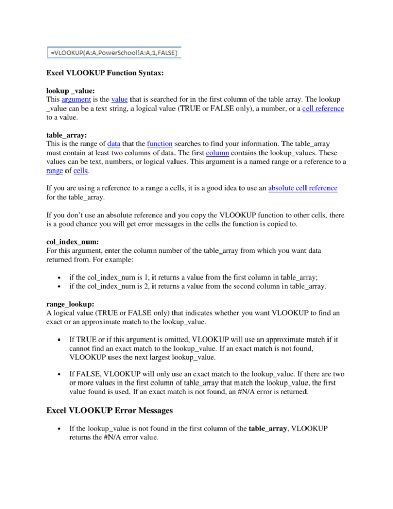
Excel VLOOKUP Function Syntax:
lookup _value:
This argument is the value that is searched for in the first column of the table array. The lookup
_value can be a text string, a logical value (TRUE or FALSE only), a number, or a cell reference
to a value.
table_array:
This is the range of data that the function searches to find your information. The table_array
must contain at least two columns of data. The first column contains the lookup_values. These
values can be text, numbers, or logical values. This argument is a named range or a reference to a
range of cells.
If you are using a reference to a range a cells, it is a good idea to use an absolute cell reference
for the table_array.
If you don’t use an absolute reference and you copy the VLOOKUP function to other cells, there
is a good chance you will get error messages in the cells the function is copied to.
col_index_num:
For this argument, enter the column number of the table_array from which you want data
returned from. For example:
•
•
if the col_index_num is 1, it returns a value from the first column in table_array;
if the col_index_num is 2, it returns a value from the second column in table_array.
range_lookup:
A logical value (TRUE or FALSE only) that indicates whether you want VLOOKUP to find an
exact or an approximate match to the lookup_value.
•
If TRUE or if this argument is omitted, VLOOKUP will use an approximate match if it
cannot find an exact match to the lookup_value. If an exact match is not found,
VLOOKUP uses the next largest lookup_value.
•
If FALSE, VLOOKUP will only use an exact match to the lookup_value. If there are two
or more values in the first column of table_array that match the lookup_value, the first
value found is used. If an exact match is not found, an #N/A error is returned.
Excel VLOOKUP Error Messages
•
If the lookup_value is not found in the first column of the table_array, VLOOKUP
returns the #N/A error value.
•
•
•
Excel's HLOOKUP function, short for horizontal lookup, is used to find specific
information that has been stored in a spreadsheet table.
HLOOKUP works much the same the Excel VLOOKUP function, or Vertical Lookup.
The only difference being that VLOOKUP searches for data in columns and HLOOKUP
searches for data in rows.
•
If the col_index_num argument is greater than the number of columns in table_array,
VLOOKUP returns the #REF! error value.
•
If the table_array argument includes empty columns on the left of the table_array,
VLOOKUP returns the #N/A error value.
Let get started!
1. Have the data you are working with on one worksheet. Have the data you are pulling you
vlooup from in another worksheet.
2. Make sure the data you are matching is in the first column. Make sure you sort the data
in first column of both worksheets in alphabetic order.
3. Click on the ScheduleStar worksheet and click next to the first record in column C.
4. Click on the Formula Tab
5. Click Insert Function
6. Click on the spreadsheet button to the right of the Lookup_value box. Choose the range.
7. Click on the spreadsheet button to the right of the Table_array box. Click on the
worksheet Powerschool now choose your range.
8. Take a look at what filled in the box not just the range but the location of Powerschool
this is telling the formula to look at the worksheet PowerSchol and use the range within
that worksheet.
9. Type 1 in Col_index_num (you are telling it to look at column 1)
10. Type False in Range_lookup (you are telling it you want an exact match)
11. You can also use True for an approximate match.
12. Fill down using the + now double click
13. Now let’s filter to all #N/A. Click on Row 1 outside the 1st column.
14. Click on Sort/Filter and choose Filter.
15. Uncheck Select All. Check #N/A