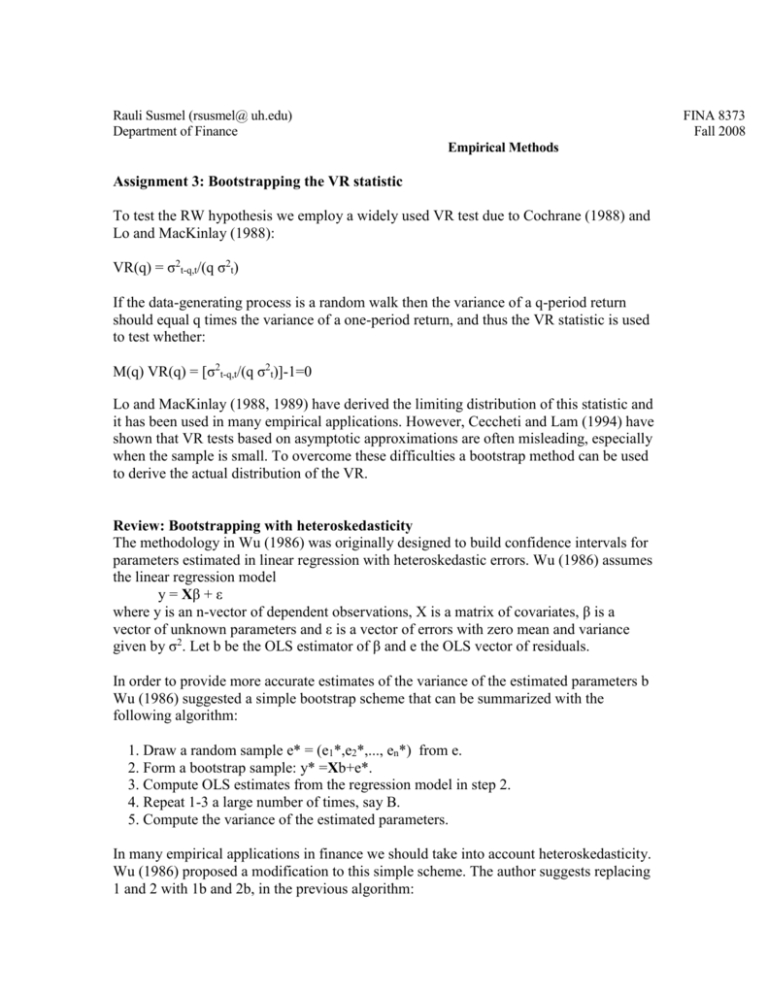
Rauli Susmel (rsusmel@ uh.edu)
Department of Finance
FINA 8373
Fall 2008
Empirical Methods
Assignment 3: Bootstrapping the VR statistic
To test the RW hypothesis we employ a widely used VR test due to Cochrane (1988) and
Lo and MacKinlay (1988):
VR(q) = σ2t-q,t/(q σ2t)
If the data-generating process is a random walk then the variance of a q-period return
should equal q times the variance of a one-period return, and thus the VR statistic is used
to test whether:
M(q) VR(q) = [σ2t-q,t/(q σ2t)]-1=0
Lo and MacKinlay (1988, 1989) have derived the limiting distribution of this statistic and
it has been used in many empirical applications. However, Ceccheti and Lam (1994) have
shown that VR tests based on asymptotic approximations are often misleading, especially
when the sample is small. To overcome these difficulties a bootstrap method can be used
to derive the actual distribution of the VR.
Review: Bootstrapping with heteroskedasticity
The methodology in Wu (1986) was originally designed to build confidence intervals for
parameters estimated in linear regression with heteroskedastic errors. Wu (1986) assumes
the linear regression model
y = Xβ + ε
where y is an n-vector of dependent observations, X is a matrix of covariates, β is a
vector of unknown parameters and ε is a vector of errors with zero mean and variance
given by σ2. Let b be the OLS estimator of β and e the OLS vector of residuals.
In order to provide more accurate estimates of the variance of the estimated parameters b
Wu (1986) suggested a simple bootstrap scheme that can be summarized with the
following algorithm:
1. Draw a random sample e* = (e1*,e2*,..., en*) from e.
2. Form a bootstrap sample: y* =Xb+e*.
3. Compute OLS estimates from the regression model in step 2.
4. Repeat 1-3 a large number of times, say B.
5. Compute the variance of the estimated parameters.
In many empirical applications in finance we should take into account heteroskedasticity.
Wu (1986) proposed a modification to this simple scheme. The author suggests replacing
1 and 2 with 1b and 2b, in the previous algorithm:
1b. For each i, draw a value ti from a distribution with zero mean and unit variance.
2b. Form a bootstrap sample: y* =Xb + ti ei/(1-wii)1/2 , i = 1,…n,
where wi = xi’(X’X)-1xi.
Cribari and Zarkos (1999) evaluated the performance of this bootstrap methodology by
comparing the weighted with the unweighted bootstrap. Their results suggest that
weighted bootstrap estimators performed very well, outperforming other estimators, even
in the case of homoskedastic errors. Even in the case of non-normality (fat tails) the
weighted bootstrap outperform other estimators.
The most important difficulty with resampling schemes is that they may generate data
that are less dependent than the original data. The bootstrap is a distribution-free
randomization technique, which can be used to estimate the sampling distribution of the
VR statistic, when the distribution of the original population is unknown.
To estimate empirical quantiles for the VR the bootstrap procedure can be carried out in
three steps:
1. Draw a bootstrap sample of N observations, rt*, t=1,…,N, with replacement from the
empirical distribution of one-period returns, rt.
2. Calculate the VR*(k) from the pseudo data rt*, for k =1,…K.
3. Repeat steps 1 and 2 M times obtaining VR*(k,m),
m=1,…M.
The nonparametric implementation of Wus (1986) method can be carried by replacing (1)
with (1a) and (1b):
(1a). For each t, draw a weighting factor zt*, t=1,…,N, with replacement from the


empirical distribution of normalized returns zt = (rt- r )/SE(r) , where r is the mean return
and SE(r) is the standard deviation of returns.
(1b). Form the bootstrap sample of N observations rt*= zt*, t=1,…N, by multiplying
each observation of actual returns with its corresponding random weighting factor.
Using this procedure, resampling from normalized returns instead from actual returns, the
weighted bootstrap method accounts for the possible nonconstancy of the variance of
returns.
Assignment
Using monthly S&P 500 (1962 to 2008), calculate the VR(q) statistic for q=2, 8. Let
B=1,000.
1) Present the p-values using the usual asymptotic distribution. Present the bootstrap pvalues. What do you learn?
2) What issues can complicate your calculations? How would you solve it?
References
Cecchetti, S. G. and P. Lam (1994), P. Variance ratio tests: small-sample properties with
an application to international output data. Journal of Business and Economic Statistics,
12, p. 177-186.
Cribari-Neto, F. and S. G. Zarkos (1999), Bootstrap methods for heteroskedastic
regression models: evidence on estimation and testing. Econometric Reviews, 18, p. 211228.
Lo, A. W. and A.C. MacKinlay (1988), Stock market prices do not follow random walks:
evidence from a simple specification test. The Review of Financial Studies 1, p. 41-66.
Lo, A. W. and A.C. MacKinlay (1989). The size and power of the variance ratio test in
finite samples. Journal of Econometrics 40, p. 203-238.
Wu, C. F. J. (1986), Jackknife, bootstrap and other resampling methods in regression
analysis. Annals of Statistics, 14, p. 1261-1295.