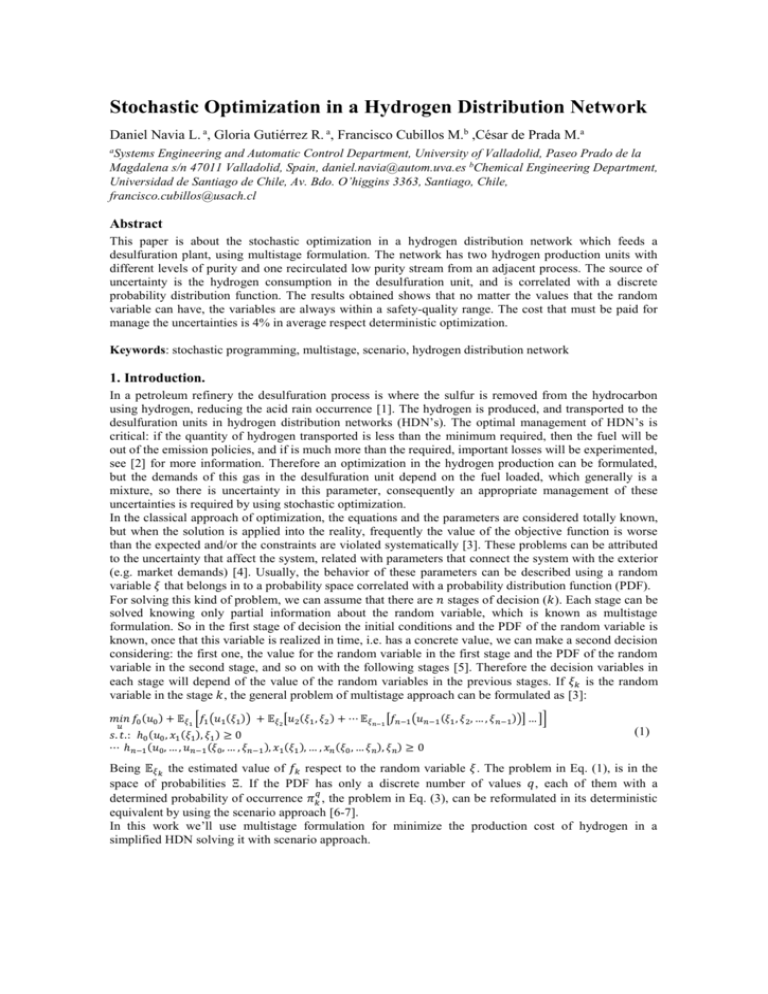
Stochastic Optimization in a Hydrogen Distribution Network
Daniel Navia L. a, Gloria Gutiérrez R. a, Francisco Cubillos M.b ,César de Prada M.a
a
Systems Engineering and Automatic Control Department, University of Valladolid, Paseo Prado de la
Magdalena s/n 47011 Valladolid, Spain, daniel.navia@autom.uva.es bChemical Engineering Department,
Universidad de Santiago de Chile, Av. Bdo. O’higgins 3363, Santiago, Chile,
francisco.cubillos@usach.cl
Abstract
This paper is about the stochastic optimization in a hydrogen distribution network which feeds a
desulfuration plant, using multistage formulation. The network has two hydrogen production units with
different levels of purity and one recirculated low purity stream from an adjacent process. The source of
uncertainty is the hydrogen consumption in the desulfuration unit, and is correlated with a discrete
probability distribution function. The results obtained shows that no matter the values that the random
variable can have, the variables are always within a safety-quality range. The cost that must be paid for
manage the uncertainties is 4% in average respect deterministic optimization.
Keywords: stochastic programming, multistage, scenario, hydrogen distribution network
1. Introduction.
In a petroleum refinery the desulfuration process is where the sulfur is removed from the hydrocarbon
using hydrogen, reducing the acid rain occurrence [1]. The hydrogen is produced, and transported to the
desulfuration units in hydrogen distribution networks (HDN’s). The optimal management of HDN’s is
critical: if the quantity of hydrogen transported is less than the minimum required, then the fuel will be
out of the emission policies, and if is much more than the required, important losses will be experimented,
see [2] for more information. Therefore an optimization in the hydrogen production can be formulated,
but the demands of this gas in the desulfuration unit depend on the fuel loaded, which generally is a
mixture, so there is uncertainty in this parameter, consequently an appropriate management of these
uncertainties is required by using stochastic optimization.
In the classical approach of optimization, the equations and the parameters are considered totally known,
but when the solution is applied into the reality, frequently the value of the objective function is worse
than the expected and/or the constraints are violated systematically [3]. These problems can be attributed
to the uncertainty that affect the system, related with parameters that connect the system with the exterior
(e.g. market demands) [4]. Usually, the behavior of these parameters can be described using a random
variable 𝜉 that belongs in to a probability space correlated with a probability distribution function (PDF).
For solving this kind of problem, we can assume that there are 𝑛 stages of decision (𝑘). Each stage can be
solved knowing only partial information about the random variable, which is known as multistage
formulation. So in the first stage of decision the initial conditions and the PDF of the random variable is
known, once that this variable is realized in time, i.e. has a concrete value, we can make a second decision
considering: the first one, the value for the random variable in the first stage and the PDF of the random
variable in the second stage, and so on with the following stages [5]. Therefore the decision variables in
each stage will depend of the value of the random variables in the previous stages. If 𝜉𝑘 is the random
variable in the stage 𝑘, the general problem of multistage approach can be formulated as [3]:
𝑚𝑖𝑛 𝑓0 (𝑢0 ) + 𝔼𝜉1 [𝑓1 (𝑢1 (𝜉1 )) + 𝔼𝜉2 [𝑢2 (𝜉1 , 𝜉2 ) + ⋯ 𝔼𝜉𝑛−1 [𝑓𝑛−1 (𝑢𝑛−1 (𝜉1 , 𝜉2 , … , 𝜉𝑛−1 ))] … ]]
𝑢
𝑠. 𝑡.: ℎ0 (𝑢0 , 𝑥1 (𝜉1 ), 𝜉1 ) ≥ 0
⋯ ℎ𝑛−1 (𝑢0 , … , 𝑢𝑛−1 (𝜉0 , … , 𝜉𝑛−1 ), 𝑥1 (𝜉1 ), … , 𝑥𝑛 (𝜉0 , … 𝜉𝑛 ), 𝜉𝑛 ) ≥ 0
(1)
Being 𝔼𝜉𝑘 the estimated value of 𝑓𝑘 respect to the random variable 𝜉. The problem in Eq. (1), is in the
space of probabilities Ξ. If the PDF has only a discrete number of values 𝑞, each of them with a
𝑞
determined probability of occurrence 𝜋𝑘 , the problem in Eq. (3), can be reformulated in its deterministic
equivalent by using the scenario approach [6-7].
In this work we’ll use multistage formulation for minimize the production cost of hydrogen in a
simplified HDN solving it with scenario approach.
Stochastic Optimization in a Hydrogen Distribution Network
2. Problem Formulation.
Let’s consider a simplified structure of a HDN represented in Figure 1 that has one desulfuration unit
(HD3), two hydrogen production units that produces with different levels of purities (H4 and H3), one
low purity recirculated stream that came from other process (UNI), and collectors connecting the
production and recirculation units with the desulfuration ones (CH4, CH3 and CBP).
Undesulfurized
Fuel m
mkCH4_HD3(x1,…,xk)
Desulfurized Fuel
HD3
CHARGE(HD3,xk)
mkHD3(x1,…,xk)
mkCBP_HD3(x1,…,xk)
mkCH3_HD3(x1,…,xk)
PkCH4(x1,…,xk)
CH4
PkCH3(x1,…,xk)
CH3
mkCH4(x1,…,xk)
mkCH3(x1,…,xk)
uk(H4,CH4)(x1,…,xk)
uk(H3,CH3)(x1,…,xk)
H4
PkCBP(x1,…,xk)
CBP
H3
mkCBP(x1,…,xk)
uk(UNI,CBP)(x1,…,xk)
UNI
Figure 1: Process flow sheet for a simplified HDN
The HDN works in stationary state because is a continuous process, but due the uncertainties that affect
the system, the problem formulation will be pseudo-stationary i.e.: for each decision stage, the hydrogen
demand can change according to its PDF.
Defining the following elements for the optimization:
Sets
· 𝑃𝑈: Production and recirculation units.
· 𝐶𝑈: Consumption units.
· 𝐶𝐿: Hydrogen Collectors.
· 𝑆𝑇𝑅: Process streams.
· 𝜉𝑘 : Random variable in each decision stage: 𝑘 = 1, … , 𝑛.
· 𝑂𝑃𝑈(𝑃𝑈, 𝐶𝐿): Process streams that comes out from 𝑃𝑈 to 𝐶𝐿.
· 𝑂𝐶𝐿(𝐶𝐿, 𝑆𝑇𝑅): Process streams that come out from 𝐶𝐿 to 𝐶𝑈.
· 𝐼𝐶𝑈(𝐶𝑈, 𝑆𝑇𝑅): Process streams that come into 𝐶𝑈.
Parameters
𝐿𝑂𝑊
𝑈𝑃
· 𝑄𝑃𝑈
, 𝑄𝑃𝑈
: Lower and Upper hydrogen molar flow production in each 𝑃𝑈
· 𝑥𝑃𝑈 Available hydrogen purity in each 𝑃𝑈
· 𝐶𝑃𝑈 : Cost of produce hydrogen in each 𝑃𝑈
𝐿𝑂𝑊
· 𝑥𝐶𝑈
Minimal mole fraction allowed for the desulfuration process.
0
· 𝑃𝐶𝐿
Initial pressure in 𝐶𝐿.
𝐿𝑂𝑊
𝑈𝑃
· 𝑃𝐶𝐿
, 𝑃𝐶𝐿
: Minimal and maximal pressures allowed respectively in each 𝐶𝐿.
· 𝑉𝐶𝐿 , 𝑇𝐶𝐿 : Volume and temperature of the collectors.
Uncertain Parameter
𝑘
(𝐶𝑈, 𝜉𝑘 ): Flow of hydrogen needed for the desulfuration in each stage.
· 𝑚𝐶𝐻𝐴𝑅𝐺𝐸
Positive Variables
· 𝑥𝑆𝑇𝑅 Hydrogen mole fraction in process streams.
𝑘 (𝜉
· 𝑚𝑆𝑇𝑅
1 , … 𝜉𝑘 ): Molar flow in process streams, upstream collectors, in stage 𝑘 = 1 … 𝑛.
𝑘
· 𝑢(𝑃𝑈,𝐶𝐿) (𝜉1 , … 𝜉𝑘 ): Molar flow produced in each 𝑃𝑈 to 𝐶𝐿, in the stage 𝑘 = 1 … 𝑛 − 1.
0
· 𝑢(𝑃𝑈,𝐶𝐿)
: Molar flow produced in each 𝑃𝑈 to 𝐶𝐿, in the first decision stage.
· 𝑥𝐶𝐿 Hydrogen mole fraction in 𝐶𝐿.
𝑘 (𝜉
· 𝑚𝐶𝐿
1 , … , 𝜉𝑘 ): Molar flow that come into each 𝐶𝐿, in the stage 𝑘 = 1, … , 𝑛 − 1.
0
· 𝑚𝐶𝐿 : Molar flow that come into each 𝐶𝐿, in the first decision stage.
𝑘 (𝜉
· 𝑃𝐶𝐿
1 , … , 𝜉𝑘 ): Pressure in 𝐶𝐿 at the end of the stage 𝑘 = 1, … , 𝑛.
𝑘 (𝜉
· 𝑥𝐶𝑈 1 , … , 𝜉𝑘 ): Hydrogen mole fraction of the stream that come into 𝐶𝑈, in the stage 𝑘 = 1, … , 𝑛
𝑘 (𝜉
· 𝑚𝐶𝑈
1 , … , 𝜉𝑘 ): Molar flow of the stream that come into 𝐶𝑈, in the stage 𝑘 = 1, … , 𝑛.
Free Variables
· 𝐴𝑘𝐶𝐿 (𝜉1 , … , 𝜉𝑘 ): Mole accumulation in each 𝐶𝐿, in stage 𝑘 = 1, … , 𝑛
𝑘 (𝐶𝐿,
· Δ𝑛𝐶𝐿
𝜉1 , … , 𝜉𝑘 ): Quantity of mole accumulated in each 𝐶𝐿, in stage 𝑘 = 1, … , 𝑛
Stochastic Optimization in a Hydrogen Distribution Network
Equations
· Mole balance at the entrance of the collector: the molar flow entering in the collector is equal to the
sum of molar flows that come from production units.
𝑘
𝑘 (𝐶𝐿,
(𝜉1 , … , 𝜉𝑘 ) = 𝑚𝐶𝐿
∑ 𝑢(𝑃𝑈,𝐶𝐿)
𝜉1 , … , 𝜉𝑘 )
𝑈𝑃∈𝑂𝑃𝑈
0
0 (𝐶𝐿),
∑ 𝑢(𝑃𝑈,𝐶𝐿)
= 𝑚𝐶𝐿
∀𝐶𝐿, 𝑘 = 1, … , 𝑛 − 1
(2)
𝐶𝐿∈𝑂𝑃𝑈
· Mole balance in the collector: due the different values that the random variable can have, the mole
balance in this unit is pseudo-stationary and the difference between the flows produced and consumed is
the mole accumulation.
𝑘 (𝜉
𝑚𝐶𝐿
1 , … , 𝜉𝑘 ) −
∑
𝑘+1 (𝜉
𝑘+1
𝑚𝑆𝑇𝑅
1 , … , 𝜉𝑘+1 ) = 𝐴𝐶𝐿 (𝜉1 , … , 𝜉𝑘+1 )
𝑆𝑇𝑅 ∈ 𝑂𝐶𝐿
0
𝑚𝐶𝐿
−
1 (𝜉 )
1
𝑚𝑆𝑇𝑅
1 = 𝐴𝐶𝐿 (𝜉1 ), ∀𝐶𝐿, 𝑘 = 1, … , 𝑛 − 1
∑
(3)
𝑆𝑇𝑅 ∈ 𝑂𝐶𝐿
The mole accumulation formulated in Eq. (6) affects the pressure inside the collectors. The change in this
variable is proportional to accumulation time 𝜃 and the difference between inner and outer flows. Ideal
Gas Law is used (in operational conditions implies a maximal error of 2.5% [8]).
𝑘 (𝜉
𝑚𝐶𝐿
1 , … , 𝜉𝑘 ) −
0
𝑚𝐶𝐿
−
∑
𝑆𝑇𝑅 ∈ 𝑂𝐶𝐿
∑
𝑉
𝐶𝐿
𝑘+1 (𝜉
𝑘+1
𝑘
𝑚𝑆𝑇𝑅
1 , … , 𝜉𝑘+1 ) = 𝜃𝑅𝑇 [𝑃𝐶𝐿 (𝜉1 , … , 𝜉𝑘+1 ) − 𝑃𝐶𝐿 (𝜉1 , … , 𝜉𝑘 )]
𝑆𝑇𝑅 ∈ 𝑂𝐶𝐿
𝑉𝐶𝐿
1 (𝜉 )
1
𝑚𝑆𝑇𝑅
1 = 𝜃𝑅𝑇 [𝑃𝐶𝐿 (𝜉1 ) −
𝐶𝐿
𝐶𝐿
0 ],
𝑃𝐶𝐿
∀𝐶𝐿, 𝑘 = 1, … , 𝑛 − 1
(4)
· Pressure bounds: For safety reasons, the pressure inside the collector must be bounded.
𝐿𝑂𝑊
𝑘 (𝜉
𝑈𝑃
𝑃𝐶𝐿
≤ 𝑃𝐶𝐿
1 , … , 𝜉𝑘 ) ≤ 𝑃𝐶𝐿 , ∀𝐶𝐿, 𝑘 = 1, … , 𝑛
(5)
· Mole Balance at the entrance of the consumption unit:
𝑘 (𝜉
𝑘
𝑚𝑆𝑇𝑅
1 , … , 𝜉𝑘 ) = 𝑚𝐶𝑈 (𝜉1 , … , 𝜉𝑘 ), ∀𝐶𝑈, 𝑘 = 1 … 𝑛
∑
(6)
𝑆𝑇𝑅∈𝐼𝐶𝑈
· Hydrogen balance at the entrance of the consumption unit:
∑
𝑘 (𝜉
𝑘
𝑘
𝑚𝑆𝑇𝑅
1 , … , 𝜉𝑘 ) 𝑥𝑆𝑇𝑅 (𝑆𝑇𝑅) = 𝑚𝐶𝑈 (𝜉1 , … , 𝜉𝑘 )𝑥𝐶𝑈 (𝜉1 , … , 𝜉𝑘 ), ∀𝐶𝑈, 𝑘 = 1 … 𝑛
(7)
𝑆𝑇𝑅∈𝐼𝐶𝑈
· Minimal purity allowed in the consumption units: The mole fraction of the stream that enters into the
consumption unit must be at least grater than a lower bound.
𝑘 (𝜉
𝐿𝑂
𝑥𝐶𝑈
1 , … , 𝜉𝑘 ) ≥ 𝑥𝐶𝑈 , ∀𝐶𝑈, 𝑘 = 1, … , 𝑛
(8)
· Minimal hydrogen flow in the consumption units: The hydrogen flow that enters into the desulfuration
unit, must be at least the one required for the desulfuration.
𝑘 (𝜉
𝑘
𝑘
𝑚𝐶𝑈
1 , … , 𝜉𝑘 )𝑥𝐶𝑈 (𝜉1 , … , 𝜉𝑘 ) ≥ 𝑚𝐶𝐻𝐴𝑅𝐺𝐸 (𝐶𝑈, 𝜉𝑘 ), ∀𝐶𝑈, 𝑘 = 1, … 𝑛
(9)
· Purity relationships:
𝑥𝑃𝑈 = 𝑥𝐶𝐿 , ∀(𝐶𝐿, 𝑃𝑈) ∈ 𝑂𝑃𝑈
𝑥𝐶𝐿 = 𝑥𝑆𝑇𝑅 , ∀(𝐶𝐿, 𝑆𝑇𝑅) ∈ 𝑂𝐶𝐿
(10)
· Lower and upper production: operational constraint about production capacity
𝐿𝑂𝑊
𝑄𝑃𝑈
≤
𝑈𝑃
𝑘 (𝜉
∑ 𝑢𝑃𝑈
1 , … , 𝜉𝑘 ) ≤ 𝑄𝑃𝑈
𝐶𝐿∈𝑂𝑃𝑈
𝐿𝑂𝑊
𝑄𝑃𝑈
≤
0
𝑈𝑃
∑ 𝑢𝑃𝑈
≤ 𝑄𝑃𝑈
, ∀𝑃𝑈, 𝑘 = 1, … , 𝑛
𝐶𝐿∈𝑂𝑃𝑈
(11)
Stochastic Optimization in a Hydrogen Distribution Network
· Cost of production: the cost of hydrogen production is calculated by using the estimated value for each
scenario in every decision stage, just like the expressed in Eq. (1) .
𝐶𝑜𝑠𝑡 =
0
∑ [𝑢(𝑃𝑈,𝐶𝐿)
𝑥𝑃𝑈 𝐶𝑃𝑈 ]
(𝑃𝑈,𝐶𝐿)
+ 𝔼𝜉1 [ ∑ 𝑢1(𝑃𝑈,𝐶𝐿) (𝜉1 )𝑥𝑃𝑈 𝐶𝑃𝑈 + ⋯
(12)
(𝑃𝑈,𝐶𝐿)
𝑛−1
(𝜉1 , … , 𝜉𝑛−1 )𝑥𝑃𝑈 𝐶𝑃𝑈 ] …]
+ 𝔼𝜉𝑛−1 [ ∑ 𝑢(𝑃𝑈,𝐶𝐿)
(𝑃𝑈,𝐶𝐿)
So the stochastic optimization problem can be summarized as: minimize Eq. (12), subject to Eq. (2) to
(11).
3. Results and discussion.
The model was programmed using 3 stages of decision in GAMS™, with CONOPT™ as NLP solver in a
computer with Intel Pentium Dual™ T2080 1.73Ghz processor and 2Gb RAM memory. The CPU time
was 0.059s with 23 variables and 24 constraints. The optimization was solved using the values of the
parameters given in Table 1, and the DPDF of the random variable represented in Figure 2. The lower
bound for the purity in the consumption unit was 0.971 in mole fraction.
Table 1. Some values of the parameters used in the stochastic optimization
𝑷𝑼
𝑯𝟒
𝑯𝟑
𝑼𝑵𝑰
𝐿𝑂
𝑄𝑃𝑈
(
𝑘𝑚𝑜𝑙
0
0
0
ℎ
)
𝑈𝑃
𝑄𝑃𝑈
(
𝑘𝑚𝑜𝑙
ℎ
32245
14300
468.77
)
𝑥𝑃𝑈
0.991
0.94
0.8
𝑪(
€
𝑴𝒎𝒐𝒍𝑯𝟐
88.1
77
0
)
𝑪𝑳
𝐿𝑂 (𝑏𝑎𝑟)
𝑃𝐶𝐿
𝑈𝑃 (𝑏𝑎𝑟)
𝑃𝐶𝐿
𝑉(𝑚3 )
𝑇(𝐾)
𝑪𝑯𝟒
𝑪𝑯𝟑
𝑪𝑩𝑷
19
19
19
21
21
21
50
50
50
300
300
300
In stochastic optimization, the idea is ensure a feasible operation having in to account the possible
changes in the random variable; in particular we will focus our attention in two constraints: the pressure
in collectors and the purity at the entrance of HD3: the pressure is a safety constraint and always must be
bounded and the hydrogen purity is a quality constraint that guaranties a good performance of the
desulfuration unit.
Figure 2: Discrete PDF for hydrogen consumption
Figure 3, shows the values of purity at the entrance of the desulfuration unit. It can be see that for each
possible value that the random variable can have according to its PDF, the purity is greater than the lower
bound.
Stochastic Optimization in a Hydrogen Distribution Network
xHD3(x11,...,xkq)
2,4,2
2,4,3
2,4,4
4,4,3
4,4,4
2,4,1
2,3,4
2,3,3
2,3,2
4,4,2
xHD3(x13,...,xkq)
XUC1
XUC3
(x12,x2q,x3q)
(x11,x2q,x3q)
0.995
XUC2
2,3,1
2,1,1
1,4,4
1,4,3
1,4,2
1,4,1
1,3,4
1,3,3
1,3,2
1,3,1
1,2,4
1,2,3
1,2,2
0.96
1,2,1
0.96
1,1,4
0.965
1,1,3
0.97
0.965
2,2,4
0.975
0.97
2,2,3
0.975
2,2,2
0.985
X 0.98
2,2,1
0.985
X 0.98
1,1,2
XUC1
0.99
0.99
1,1,1
xHD3(x12,...,xkq)
0.995
XUC3
2,1,4
XUC2
2,1,3
XUC1
2,1,2
0.995
XUC2
xHD3(x14,...,xkq)
XUC1
0.995
XUC3
0.99
XUC2
XUC3
(x13,x2q,x3q)
4,4,1
4,3,4
4,3,3
4,3,2
4,3,1
4,2,4
4,2,3
4,1,1
3,4,4
3,4,3
3,4,2
3,4,1
3,3,4
3,3,3
3,3,2
3,3,1
3,2,4
3,2,3
3,2,2
3,2,1
3,1,4
0.96
3,1,3
0.96
3,1,2
0.965
3,1,1
0.97
0.965
4,2,2
0.975
0.97
4,2,1
0.975
4,1,4
0.985
X 0.98
4,1,3
0.985
X0.98
4,1,2
0.99
(x14,x2q,x3q)
Figure 3: Evolution of the purity at the entrance of the Consumption unit, for each stage
Figure 4 shows the evolution of the pressure for CH4 and CH3 in every decision stage (CBP is irrelevant,
because for all stages 𝑚𝐶𝐵𝑃_𝐻𝐷3 is in the upper bound). It can be noted that for every possible value that
the hydrogen demand can have, the pressure is always within the safety operational range.
P (bar)
21
PCH4k(x12,...,xkq)
PCL1 PCL2 PCL3
P (bar)
PCH4k(x11,...,xkq)
PCL1 PCL2 PCL3
21.5
21.5
21
P (bar)
PCH3k(x13,...,xkq)
PCL1 PCL2 PCL3
21
2,4,4
2,4,3
2,4,2
2,4,1
2,3,4
2,3,3
2,3,2
2,3,1
2,2,4
4,4,3
4,4,4
2,4,3
2,4,4
4,4,1
4,3,4
4,3,3
4,3,2
4,3,1
2,4,1
2,3,4
2,3,3
2,3,2
2,3,1
2,2,4
(x12,x2q,x3q)
(x11,x2q,x3q)
21.5
2,2,3
2,1,1
1,4,4
1,4,3
1,4,2
1,4,1
1,3,4
1,3,3
1,3,2
1,3,1
1,2,4
1,2,3
1,2,2
1,2,1
1,1,4
1,1,3
19
18.5
1,1,2
19
18.5
2,2,2
20
19.5
2,2,1
20
19.5
2,1,4
21
20.5
2,1,3
21
1,1,1
PCH3k(x12,...,xkq)
PCL1 PCL2 PCL3
21.5
20.5
P (bar)
4,4,2
P (bar)
2,1,2
21.5
4,2,4
(x14,x2q,x3q)
PCH3k(x11,...,xkq)
PCL1 PCL2 PCL3
P (bar)
2,4,2
(x13,x2q,x3q)
4,2,3
4,1,1
3,4,4
3,4,3
3,4,2
3,4,1
3,3,4
3,3,3
3,3,2
3,3,1
3,2,4
3,2,3
3,2,2
3,2,1
3,1,4
3,1,3
3,1,2
19
18.5
3,1,1
19
18.5
4,2,1
20
19.5
4,1,4
20
19.5
4,1,3
21
20.5
4,1,2
21
20.5
(a)
PCH4k(x14,...,xkq)
PCL1 PCL2 PCL3
21.5
4,2,2
PCH4k(x13,...,xkq)
PCL1 PCL2 PCL3
21.5
2,2,3
(x12,x2q,x3q)
(x11,x2q,x3q)
P (bar)
2,2,2
2,2,1
2,1,1
1,4,4
1,4,3
1,4,2
1,4,1
1,3,4
1,3,3
1,3,2
1,3,1
1,2,4
1,2,3
1,2,2
1,2,1
1,1,4
1,1,3
1,1,2
19
18.5
1,1,1
19
18.5
2,1,4
20
19.5
2,1,3
20
19.5
2,1,2
20.5
20.5
(b)
PCH3k(x14,...,xkq)
PCL1 PCL2 PCL3
P (bar)
21.5
21
20.5
(x13,x2q,x3q)
4,4,4
4,4,3
4,4,2
4,4,1
4,3,4
4,3,3
4,3,2
4,3,1
4,2,4
4,2,3
4,2,2
4,2,1
4,1,4
3,4,4
3,4,3
3,4,2
3,4,1
3,3,4
3,3,3
3,3,2
3,3,1
3,2,4
3,2,3
3,2,2
3,2,1
3,1,4
3,1,3
3,1,2
19
18.5
3,1,1
19
18.5
4,1,3
20
19.5
4,1,2
20
19.5
4,1,1
20.5
(x14,x2q,x3q)
Figure 4: Evolution of the Pressures inside the collectors (a) CH4 and (b) CH3, for each stage
Stochastic Optimization in a Hydrogen Distribution Network
It’s important to mention that the feasible operation is only ensured for the values considered in discrete
PDF because the scenario formulation.
Finally, Table 2 lists the estimated value of the hydrogen production cost obtained with stochastic
approach and the one calculated by deterministic optimization using the expected value of the hydrogen
demand. It can be seen that the estimated value of the objective function in stochastic optimization is 4%
in average greater than the deterministic result for all the stages considered, which can be understood as
the cost that must be paid to manage the uncertainties.
Table 2. Costs obtained with stochastic and deterministic optimization
Stochastic
Stage
0
1
2
Est. Cost (€⁄ℎ)
878.04
810.71
810.24
Cost (€⁄ℎ)
Deterministic
821.47
4. Conclusions
The use of discrete PDF allows solving the stochastic problem like a deterministic one, but we can
guarantee a feasible operation respect to critical variables in a simplified model of HDN (collector
pressure and hydrogen purity) only for the values considered. If the solution must be more robust, then
more values in the PDF have to be considered, with the corresponding rise in computational effort. The
average cost that must be paid for handle the uncertainties is 4% respect to the deterministic optimization.
5. Acknowledgements
Erasmus Mundus External Cooperation Window Lot 17 (EMECW Lot 17)
References
[1] Larssen, T. and G.R. Carmichael, Env. Pollut., 2000. 110(1): p. 89-102.
[2] Sarabia, D., et al., in Proceedings of ADCHEME. 2009: Istambul, Turkey.
[3] Rockafellar, R.T. (2001) Optimization Under Uncertainty.
[4] Wendt, M., P. Li, and G. Wozny, Ind. Eng. Chem. Res., 2002. 41(15): p. 3621-3629.
[5] Dantzig, G.B., LINEAR PROGRAMMING UNDER UNCERTAINTY. Management Science, 1955. 1(3-4): p.
197-206.
[6] Birge, J.R. and F. Louveaux, Introduction to stochastic programming. Springer series in operations research. 1997,
New York: Springer. xix, 421 p.
[7] Ruszczynski, A. and A. Shapiro, Stochastic Programming Models, in Handbooks in Operations Research and
Management Science, A. Ruszczynski and A. Shapiro, Editors. 2003, Elsevier.
[8] Çengel, Y.A. and M.A. Boles, Thermodynamics : an engineering approach. 5th ed. McGraw-Hill series in
mechanical engineering. 2006, Boston: McGraw-Hill Higher Education. xxxvi