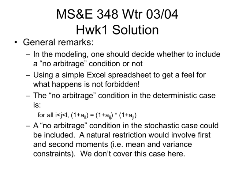
MS&E 348 Wtr 03/04
Hwk1 Solution
• General remarks:
– In the modeling, one should decide whether to include
a “no arbitrage” condition or not
– Using a simple Excel spreadsheet to get a feel for
what happens is not forbidden!
– The “no arbitrage” condition in the deterministic case
is:
for all i<j<l, (1+ail) = (1+aij) * (1+ajl)
– A “no arbitrage” condition in the stochastic case could
be included. A natural restriction would involve first
and second moments (i.e. mean and variance
constraints). We don’t cover this case here.
1. Deterministic Case
Min z
x
s.t. x12 + x13 + x14 – s1 = b1
x23 + x24 + (s1-x12) (1+a12) – s2 = b2
x34 + (s2 – x23) (1+a23) – x13 (1+a13) – s3 = b3
x14 (1+a14) + x24 (1+a24) + x34 (1+a34) – s3 (1+a34) = z
xij ≥ 0 decision variables, si ≥ 0 slack variables
bi liabilities & aij interest rates are given
Excel formulation: no “arb”
Time
1
2
3
4
External Liability
b1
100.00
b2
100.00
b3
100.00
Amount Borrowed
x12
x13
x14
100.00
-
x23
x24
210.00
-
x34
331.00
Debt Due
from
Previous Borrowings
Term Structure
Net CF
From t=1
1+a12
1+a13
1+a14
1.10
1.21
1.33
-
1+a23
1+a24
110
1.10
1.21
-
From t=1
" t=2
1+a34
0
231
-
From t=1
" t=2
" t=3
0
0
364.1
1.10
-
z
364.10
Given the consistency of the term structure, there’s an infinity of solutions
all giving the same borrowing costs (at t=4) equal to z = 364.1 for the chosen
parameters values.
Excel formulation: with “arb”
Time
1
2
External Liability
b1
100.00
b2
Amount Borrowed
x12
x13
x14
100.15
-
x23
x24
Debt Due
from
Previous Borrowings
Term Structure
Net CF
From t=1
1+a12
1+a13
1+a14
1.10
1.21
1.33
0.15
1+a23
1+a24
3
100.00
48,806,747.45
110.1703395
1.10
1.11
48,806,537.45
4
b3
100.00
x34
-
From t=1
" t=2
0
0
1+a34
-
From t=1
" t=2
" t=3
0
54175489.67
0
1.10
53,687,091.20
z (4,880,310.65)
Here 1 + a24 has been modified and set to 1.11 < (1+a23) (1+a34) = 1.21
Solver does not converge and model “blows up”!
As expected you would borrow a huge amount x24 at t=2 and make money
by rolling over the surplus from one period to the next!
2. Stochastic Case
Min E[zw2w3]
x
s.t. x12 + x13 + x14 – s1 = b1
X23w2 + x24w2 + (s1-x12) (1+a12) – s2w2 = b2
x34w2w3 + (s2w2 – x23w2) (1+a23w2) – x13 (1+a13) – s3w2w3 = b3
x14 (1+a14) + x24w2 (1+a24w2) + x34w2w3 (1+a34w2w3) – s3w2w3 (1+a34w2w3) = zw2w3
Xijw ≥ 0 decision variables, siw ≥ 0 slack variables
bi liabilities & aijw interest rates are given
One of the modeling decisions here was to decide whether a13 and a14
should be uncertain or not. Here we assume these rates are
deterministic like a12.
3. Utility Function
There’s no one answer to this question as long as you’re consistent
For instance, based upon expected values of interest rates, one could
compute an approximate “expected” value of the total borrowing costs
zE incurred at time t=4 to cover all previous borrowings
Then one could apply a (dis)utility function that strongly penalizes incurring
borrowing costs higher than this base value
U(z)
Piecewise linear
C1
zE
Base value
z
Make sure the shape and orientation of the utility curve you use is consistent
with the fact that you want to minimize borrowing costs!