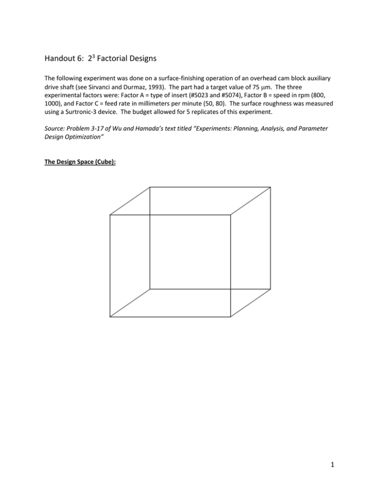
Handout 6: 23 Factorial Designs
The following experiment was done on a surface-finishing operation of an overhead cam block auxiliary
drive shaft (see Sirvanci and Durmaz, 1993). The part had a target value of 75 m. The three
experimental factors were: Factor A = type of insert (#5023 and #5074), Factor B = speed in rpm (800,
1000), and Factor C = feed rate in millimeters per minute (50, 80). The surface roughness was measured
using a Surtronic-3 device. The budget allowed for 5 replicates of this experiment.
Source: Problem 3-17 of Wu and Hamada’s text titled “Experiments: Planning, Analysis, and Parameter
Design Optimization”
The Design Space (Cube):
1
There are 2^3 = 8 corners in this design space. These types of experiments are often considered
screening designs. The Low and High limit for each factor are often set at the most extreme levels for
which the process can operate.
There is some general notation that is used for this type of experiment. The following is considered
standard notation.
The design points are labeled as follows…
A
B
C
Notation
-
-
-
(1)
+
-
-
A
-
+
-
B
-
-
+
C
+
+
-
AB
+
-
+
AC
-
+
+
BC
+
+
+
ABC
2
Setting up the Design in Minitab:
Select Stat > DOE > Factorial > Create Factorial Design…
Under Number of factors, select 3 as we have three factors (i.e., we have a 2^3 experiment).
3
Under the Display Available Designs... tab we find the following:
Design Resolution is an issue when you cannot run a “full” set of design points. For example, if we have
four factors each at 2 levels (2^4 = 16), but can only run 8 design points for some reason, then we have a
fractionated design. When a design is fractionated, design resolution is used to differentiate between
the quality of such designs. As a general rule, the larger the design resolution, the better the design.
Design resolution is discussed in some detail in Section 8.2.2 of our textbook.
For our experiment, we are able to run all 2^3=8 design points. As a result, click on the Designs… tab
and select Full factorial. Also, we will run 5 replicates at each design point, so select 5 under Number of
replicates for corner points.
4
Under the Factors… tab we can specify labels for each of our factor levels. The default codings are -1
and +1 for Low and High levels, respectively. We can specify Insert Type (#5023 and #5074), Speed (800,
1000), and Feed Rate (50, 80).
Default Coding…
Changing the Default Coding under the Factors
Tab…
Notice, the factor levels are now coded…
Additional items can be specified under the Options and Results tabs:
The following items are found under the Options…
tab
The following items are found under the
Results… tab
5
After you have setup your design, you can make changes, modify, or display the design under the DOE
submenu.
The data from our experiment (from Wu and Hamada, Problem 3-17):
A
#5023
#5023
#5023
#5023
#5074
#5074
#5074
#5074
Factors
B
800
800
1000
1000
800
800
1000
1000
C
50
80
50
80
50
80
50
80
Rep 1
54.6
86.2
41.4
62.8
59.6
82.0
43.4
65.6
Rep 2
73
66.2
51.2
64.8
52.8
72.8
49.0
65.0
Roughness
Rep 3
139.2
79.2
42.6
74.6
55.2
76.6
48.6
64.2
Rep 4
55.4
86
58.6
74.6
61.0
73.4
49.6
60.8
Rep 5
52.6
82.6
58.4
64.6
61.0
75.0
55.2
77.4
6
A portion of the data in Minitab…
The Analysis
If you have set up the design in Minitab, then you can simply click on Stat> DOE > Factorial > Analyze
Factorial Design… If you have not setup your design in Minitab, you may have to use Stat > ANOVA >
General Linear Model… to analyze your data.
In the first window, we must specify the response variable. In this experiment, the response variable or
outcome variable of interest is Roughness.
7
Under the Terms… tab, we must specify the terms we want to put in our model. Initially, we should put
all main effects (A, B, and C) in our model. We should also include the two-way interaction terms in our
model (AB, AC, and BC). The two-way interactions will allow for the effect of one variable to change
depending on the level of a second variable. If the two-way interactions are not included in the model,
then you are forcing the effect of A to be the same across the levels of B and C. Similarly, the three-way
interaction, ABC, will be included in an initial model.
Under the Graphs… tab, select Normal under Effects Plots (this will give us a visualization of the
importance of each estimated model effect) and select Four in one under Residuals plots.
8
Under the Results… tab, specify each model effect under Display of Least Squares Means. This will
estimate the effect for each factor level combination in our experiment.
Finally, under the Storage… tab, select Fits and Residuals.
Note: The leverage, Cook’s distance, and DFITS are not selected here, but can be used to identify
observations that may adversely affect our model.
9
The Output from Minitab…
The following is a list of p-values for each of the model effects. When investigating the importance of
each effect, make sure and use the “bottom-up” approach. That is, make sure there is NOT significant
three-way interaction before considering any two-way interactions. Likewise, make sure the effects of
all two-way interactions are negligible before considering the main effects.
A normal probability plot of the standardized estimated model effects is given here. Significant effects
are those that “fall off the line”. This method is somewhat subjective, and I do not advocate using this
method to identify significant effects.
10
Minitab gives the following additional output that tests the importance of the Main Effects, 2-Way
Interactions, and 3-Way Interactions. To be honest, these tests are not normally used in practice.
•
There is one 3-Way Interaction term in our model, and the table above displays the same test for
the three-way interaction as before (df=1, p=0.462).
•
There are three 2-Way Interaction terms in our model (AB, AC, and BC). These three 2-Way
Interaction tests are combined into one test in the output above (e.g. df=3, 1 + 1 + 1). This test is
getting at the “overall effect” of the 2-Way interactions.
•
Likewise, there are three main effects (A, B, and C) in our experiment. These three main effects are
combined into one test in the output above. Again, this test is getting at the “overall effect” of
these three factors.
11
The Estimated Model Coefficients…
The estimated coefficients (in the uncoded units) are given here. These are used to compute the Least
Squares Means (i.e. the best-guess for Roughness for various factor level combinations in our
experiment).
The coefficients above can be used to build a prediction equation as follows.
𝑃𝑟𝑒𝑑𝑖𝑐𝑡𝑒𝑑 𝑅𝑜𝑢𝑔ℎ𝑛𝑒𝑠𝑠
=
154.3
+ (−95.4 ∗ 𝐼𝑛𝑠𝑒𝑟𝑡 𝑇𝑦𝑝𝑒) + (−0.13 ∗ 𝑆𝑝𝑒𝑒𝑑) + (−0.42 ∗ 𝐹𝑒𝑒𝑑 𝑅𝑎𝑡𝑒)
+ (0.095 ∗ 𝐼𝑛𝑠𝑒𝑟𝑡 𝑇𝑦𝑝𝑒 ∗ 𝑆𝑝𝑒𝑒𝑑) + (1.11 ∗ 𝐼𝑛𝑠𝑒𝑟𝑡 𝑇𝑦𝑝𝑒 ∗ 𝐹𝑒𝑒𝑑 𝑅𝑎𝑡𝑒)
+ (0.001 ∗ 𝑆𝑝𝑒𝑒𝑑 ∗ 𝐹𝑒𝑒𝑑 𝑅𝑎𝑡𝑒)
+ (−0.0011 ∗ 𝐼𝑛𝑠𝑒𝑟𝑡 𝑇𝑦𝑝𝑒 ∗ 𝑆𝑝𝑒𝑒𝑑 ∗ 𝐹𝑒𝑒𝑑 𝑅𝑎𝑡𝑒)
Setting this up in Excel and making a prediction for Insert Type = #5023; Speed = 800; Feed Rate = 50
The standard ANOVA table includes coefficients as well, but these can only be used with coded units, i.e.
-1 / +1 notation.
12
Predicted Roughness for all corners of design cube….
13
Checking the Residuals (i.e. validity of the model)
The unusual observations printed out by Minitab’s session window are shown below.
An examination of the residuals also identifies the outlier:
A list of the data with the predicted values (FITS1) and the Residuals (RESI1)
14
Consideration of Removing the Outlier - “Fixing” the Model
Minitab output for testing the model effects.
Questions
1. What is the effect of the outlier on the overall error in our experiment (i.e. S)?
2. What is the effect of the outlier on the p-values for testing the importance of the model effects?
That is, how did the p-values change?
The updated Normal Probability plot also suggests that Main Effect B and Main Effect C have a
significant effect on Roughness.
15
The Estimated Model Coefficients…
The estimated coefficients (in the uncoded units) for our
updated model.
The estimated coefficients for our original model.
16
Checking the Residuals (i.e. validity of the updated model)
The unusual observations…
The residuals for our updated model look better…
The following graphic shows our data with the fitted values and residuals…
17
Visualizing the Estimated Effect on Roughness
Again, if the design has been set up in Minitab, visualizations of the predicted values from our model
effects can be created easily. Select Stat > DOE > Factorial > Factorial Plots…
There are three types of plots that are available: Main Effects Plot, Interaction Plot, and Cube Plot. The
Main Effects plot should not be used if interactions are present in our model.
You must specify the setup for the plots under the Setup… tab. This is shown here for the Main Effects
plots.
18
The resulting Cube Plot from Minitab….
The resulting Main Effects Plot from Minitab:
Note: It is only appropriate to look at this plot when there are not any two-way or three-way
interactions present in our analysis.
19
The following is a display of the three two-way interaction plots that are returned by Minitab:
Additional Plotting Options…
The following plots can be used when the Factors being considered are numerical in nature (e.g. Speed =
800 and 1000, and Feed Rate = 50 and 80).
20
Select the Contour plot and/or Surface Plot.
Under the Setup… tab, specify the response variable, the factor to be used for the X Axis and the factor
to be used on the Y Axis.
Factor A is not numerical (#5023 and #5074) and thus the level of Factor A should be specified under the
Settings… tab. Below, the level of Factor A is set to #5023.
21
The following is the Surface plot returned by Minitab. This surface plot is for Insert Type = #5023 only.
Changing the Insert Type to #5074 under the Settings… tab gives the following plot:
Questions:
1. What is the apparent effect of Speed on the Roughness?
2. What is the apparent effect of Feed Rate on Roughness?
3. What is the apparent effect of Insert Type on Roughness?
4. Why can we marginalize these effects in this analysis?
22
The following is the Contour plot returned by Minitab. This contour plot is for Insert Type = #5023 only.
The following is the Contour plot for Insert Type = #5074.
23
Optimizing a Process…
Suppose that the optimal roughness for our process is 75 m. Find an optimal setting for each of the
factors to achieve this target.
Select Stat > DOE > Factorial > Response Optimizer…
In the Response Optimizer, select Roughness for the response variable.
Note: The true power of this optimizer process is its ability to optimize a process over several different
response variables.
The target of 75, a lower limit, and an upper limit should be specified under the Setup… tab.
24
The following optimizing screen is returned. The optimal setting returned by Minitab for a target of 75 is
Insert Type #5074, Speed = 800, and Feed Rate = 78.4.
If it is necessary to use Insert Type #5023, then it looks like the Speed should be increased to about 885
and the Feed Rate set at about 80. Note that the desirability value (D) for this setting is near the optimal
value of 1.0. The desirability functions are briefly discussed on page 437 of your textbook (a portion of
the Minitab help file on desirability is also shown below).
25
Suppose the current settings for our process are Insert Type = #5023, Speed=800 rpm, and Feed Rate=60
mm/min. Comment on our ability to reach the target value of 75 m.
Discussions about Desirability Functions
 See page 437 of textbook
 See below which is from the Minitab help window.
26
Fitting a Reduced Model…
In the above analysis, we discovered that the only significant factors in this process were Speed and
Feed Rate. Some advocate that a reduced model can be fit at this point. A reduced model contains only
the factors found to be significant.
To fit this reduced model, select Stat> DOE > Factorial > Analyze Factorial Design… Specify Roughness
as our Response variable and under the Terms… tab, select the significant factors (i.e. Speed and Feed
Rate).
The visualization for our reduced model involves collapsing the cube over Factor A (the non-significant
factor).
The original design cube…
The design cube collapsed over Factor A
27
The following reduced model output is returned.
Compare the reduced model output against the original model output.
Questions:
1. What is the effect of using the reduced model on the overall error in our experiment (i.e. S)?
2. What is the effect of using the reduced model on the p-values for Speed and Feed Rate?
Comment: My personal philosophy is that a reduced model should be used only for plotting the effect
of the significant factors on the response variable. I would discourage you from reporting the value of S
or the importance of the factors from the reduced model.
28
In the following plots, we can observe the effect of Speed and Feed Rate. There is no effect due to
Insert Type in this model, because this factor was not included in the reduced model.
29
The Main Effect plot and cube plot for our reduced model are given here.
There are only two factors in our reduced model as the cube has been collapsed across the other factor.
As a result, our cube has 4 unique values and not 8.
30
The following dotplot of the fitted values (or predicted values) from our reduced model displays the 4
unique values. In this plot, we can see that Speed and Feed Rate affect the response; however, Insert
Type does not as it was excluded in our reduced model.
31
Appendix for JMP
Setting up the Design
To set up this design in JMP, select DOE > Screening Designs. Specify the Roughness as the response.
You can specify Match Target as the goal. In the Factors, specify the three factors for this design. Insert
Type is categorical and Speed and Feed Rate as Continuous factors. You can specify the factor level
settings in the Values boxes.
After specifying the factors, select Choose from a list of fractional factorial designs. Click Continue.
32
Select Full Factorial. In the Output Options, specify the Number of Replicates as 4 (one less than the
number in the design).
Click Make Table. The experimental settings are returned in random order. After running the
experiment, enter the responses into your design.
33
The Analysis Step
In JMP, various analysis output can be obtained under the Screening and Model drop-down menus.
The Fit Model dialog box can be obtained by selecting Model > Run Script.
34
Model Output
The Effect Tests portion of the output contians p-values for each factor as well. The estimated
model coefficents is given above under Estimate.
35
Plots
JMP provides a single residual plot (instead of four-in-one residual plot as Minitab).
In order create surface plots and contour plots, you must first save the predicted values, i.e. means, into
your dataset. This can be done by selecting Save Columns > Prediction Formula.
36
To create a surface plot, select Graph > Surface Plot. Specify any and all numeric variables in the
Columns box.
The following window is returned. You can specify various settings in this window.
37
The Predictor Profiler can be selected from the red-drop down menu as is shown here.
38