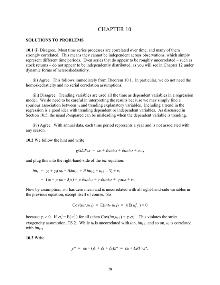
CHAPTER 10
SOLUTIONS TO PROBLEMS
10.1 (i) Disagree. Most time series processes are correlated over time, and many of them
strongly correlated. This means they cannot be independent across observations, which simply
represent different time periods. Even series that do appear to be roughly uncorrelated – such as
stock returns – do not appear to be independently distributed, as you will see in Chapter 12 under
dynamic forms of heteroskedasticity.
(ii) Agree. This follows immediately from Theorem 10.1. In particular, we do not need the
homoskedasticity and no serial correlation assumptions.
(iii) Disagree. Trending variables are used all the time as dependent variables in a regression
model. We do need to be careful in interpreting the results because we may simply find a
spurious association between yt and trending explanatory variables. Including a trend in the
regression is a good idea with trending dependent or independent variables. As discussed in
Section 10.5, the usual R-squared can be misleading when the dependent variable is trending.
(iv) Agree. With annual data, each time period represents a year and is not associated with
any season.
10.2 We follow the hint and write
gGDPt-1 = 0 + 0intt-1 + 1intt-2 + ut-1,
and plug this into the right-hand-side of the intt equation:
intt = 0 + 1(0 + 0intt-1 + 1intt-2 + ut-1 – 3) + vt
= (0 + 10 – 31) + 10intt-1 + 11intt-2 + 1ut-1 + vt.
Now by assumption, ut-1 has zero mean and is uncorrelated with all right-hand-side variables in
the previous equation, except itself of course. So
Cov(int,ut-1) = E(intt  ut-1) = 1E( ut21 ) > 0
because 1 > 0. If  u2 = E( u t2 ) for all t then Cov(int,ut-1) = 1  u2 . This violates the strict
exogeneity assumption, TS.2. While ut is uncorrelated with intt, intt-1, and so on, ut is correlated
with intt+1.
10.3 Write
y* = 0 + (0 + 1 + 2)z* = 0 + LRP  z*,
79
and take the change: y* = LRP  z*.
10.4 We use the R-squared form of the F statistic (and ignore the information on R 2 ). The 10%
critical value with 3 and 124 degrees of freedom is about 2.13 (using 120 denominator df in
Table G.3a). The F statistic is
F = [(.305  .281)/(1  .305)](124/3)
 1.43,
which is well below the 10% cv. Therefore, the event indicators are jointly insignificant at the
10% level. This is another example of how the (marginal) significance of one variable (afdec6)
can be masked by testing it jointly with two very insignificant variables.
10.5 The functional form was not specified, but a reasonable one is
log(hsestrtst) = 0 + 1t + 1Q2t + 2Q3t + 3Q3t + 1intt +2log(pcinct) + ut,
Where Q2t, Q3t, and Q4t are quarterly dummy variables (the omitted quarter is the first) and the
other variables are self-explanatory. This inclusion of the linear time trend allows the dependent
variable and log(pcinct) to trend over time (intt probably does not contain a trend), and the
quarterly dummies allow all variables to display seasonality. The parameter 2 is an elasticity
and 100  1 is a semi-elasticity.
10.6 (i) Given j = 0 + 1 j + 2 j2 for j = 0,1,
,4, we can write
yt = 0 + 0zt + (0 + 1 + 2)zt-1 + (0 + 21 + 42)zt-2 + (0 + 31 + 92)zt-3
+ (0 + 41 + 162)zt-4 + ut
= 0 + 0(zt + zt-1 + zt-2 + zt-3 + zt-4) + 1(zt-1 + 2zt-2 + 3zt-3 + 4zt-4)
+ 2(zt-1 + 4zt-2 + 9zt-3 + 16zt-4) + ut.
(ii) This is suggested in part (i). For clarity, define three new variables: zt0 = (zt + zt-1 + zt-2 +
zt-3 + zt-4), zt1 = (zt-1 + 2zt-2 + 3zt-3 + 4zt-4), and zt2 = (zt-1 + 4zt-2 + 9zt-3 + 16zt-4). Then, 0, 0, 1,
and 2 are obtained from the OLS regression of yt on zt0, zt1, and zt2, t = 1, 2, , n. (Following
our convention, we let t = 1 denote the first time period where we have a full set of regressors.)
The ˆ j can be obtained from ˆ j = ˆ0 + ˆ1 j + ˆ2 j2.
(iii) The unrestricted model is the original equation, which has six parameters (0 and the
five j). The PDL model has four parameters. Therefore, there are two restrictions imposed in
moving from the general model to the PDL model. (Note how we do not have to actually write
out what the restrictions are.) The df in the unrestricted model is n – 6. Therefore, we would
obtain the unrestricted R-squared, Rur2 from the regression of yt on zt, zt-1, , zt-4 and the
restricted R-squared from the regression in part (ii), Rr2 . The F statistic is
80
( Rur2  Rr2 ) (n  6)
F 

.
(1  Rur2 )
2
Under H0 and the CLM assumptions, F ~ F2,n-6.
SOLUTIONS TO COMPUTER EXERCISES
10.7 Let post79 be a dummy variable equal to one for years after 1979, and zero otherwise.
Adding post79 to equation 10.15) gives
i3t = 1.26 + .592 inft
(0.43) (.074)
+ .478 deft
(.154)
+ 1.41 post79t
(0.66)
n = 49, R2 = .725, R 2 = .707.
The coefficient on post79 is statistically significant (t statistic  2.14) and economically large:
accounting for inflation and deficits, i3 was about 1.4 points higher on average in years after
1979. The coefficient on def falls substantially once post79 is included in the regression.
10.8 (i) Adding a linear time trend to (10.22) gives
log (chnimp) = 2.37  .686 log(chempi) + .466 log(gas) + .078 log(rtwex)
(20.78) (1.240)
(.876)
(.472)
+
.090 befile6 + .097 affile6  .351 afdec6 + .013 t
(.251)
(.257)
(.282)
(.004)
n = 131, R2 = .362, R 2 = .325.
Only the trend is statistically significant. In fact, in addition to the time trend, which has a t
statistic over three, only afdec6 has a t statistic bigger than one in absolute value. Accounting for
a linear trend has important effects on the estimates.
(ii) The F statistic for joint significance of all variables except the trend and intercept, of
course) is about .54. The df in the F distribution are 6 and 123. The p-value is about .78, and so
the explanatory variables other than the time trend are jointly very insignificant. We would have
to conclude that once a positive linear trend is allowed for, nothing else helps to explain
log(chnimp). This is a problem for the original event study analysis.
(iii) Nothing of importance changes. In fact, the p-value for the test of joint significance of
all variables except the trend and monthly dummies is about .79. The 11 monthly dummies
themselves are not jointly significant: p-value  .59.
10.9 Adding log(prgnp) to equation (10.38) gives
81
log ( prepopt ) = 6.66  .212 log(mincovt) + .486 log(usgnpt) + .285 log(prgnpt)
(1.26) (.040)
(.222)
(.080)
 .027 t
(.005)
n = 38, R2 = .889, R 2 = .876.
The coefficient on log(prgnpt) is very statistically significant (t statistic  3.56). Because the
dependent and independent variable are in logs, the estimated elasticity of prepop with respect to
prgnp is .285. Including log(prgnp) actually increases the size of the minimum wage effect: the
estimated elasticity of prepop with respect to mincov is now .212, as compared with .169 in
equation (10.38).
10.10 If we run the regression of gfrt on pet, (pet-1 – pet), (pet-2 – pet), ww2t, and pillt, the
coefficient and standard error on pet are, rounded to four decimal places, .1007 and .0298,
respectively. When rounded to three decimal places we obtain .101 and .030, as reported in the
text.
10.11 (i) The coefficient on the time trend in the regression of log(uclms) on a linear time trend
and 11 monthly dummy variables is about .0139 (se  .0012), which implies that monthly
unemployment claims fell by about 1.4% per month on average. The trend is very significant.
There is also very strong seasonality in unemployment claims, with 6 of the 11 monthly dummy
variables having absolute t statistics above 2. The F statistic for joint significance of the 11
monthly dummies yields p-value  .0009.
(ii) When ez is added to the regression, its coefficient is about .508 (se  .146). Because
this estimate is so large in magnitude, we use equation (7.10): unemployment claims are
estimated to fall 100[1 – exp(.508)]  39.8% after enterprise zone designation.
(iii) We must assume that around the time of EZ designation there were not other external
factors that caused a shift down in the trend of log(uclms). We have controlled for a time trend
and seasonality, but this may not be enough.
10.12 (i) The regression of gfrt on a quadratic in time gives
ˆ = 107.06 + .072 t - .0080 t2
gfr
t
(6.05) (.382)
(.0051)
n = 72, R2 = .314.
Although t and t2 are individually insignificant, they are jointly very significant (p-value 
.0000).
82
(ii) Using gfrt as the dependent variable in (10.35) gives R2  .602, compared with about .727
if we do not initially detrend. Thus, the equation still explains a fair amount of variation in gfr
even after we net out the trend in computing the total variation in gfr.
(iii) The coefficient and t statistic on t3 are about .00129 and .00019, respectively, which
results in a very significant t statistic. It is difficult to know what to make of this. The cubic
trend, like the quadratic, is not monotonic. So this almost becomes a curve-fitting exercise.
10.13 (i) The estimated equation is
gct
= .0081 + .571 gyt
(.0019)
(.067)
n = 36, R2 = .679.
This equation implies that if income growth increases by one percentage point, consumption
growth increases by .571 percentage points. The coefficient on gyt is very statistically significant
(t statistic  8.5).
(ii) Adding gyt-1 to the equation gives
gct = .0064 + .552 gyt + .096 gyt-1
(.0023)
(.070)
(.069)
n = 35, R2 = .695.
The t statistic on gyt-1 is only about 1.39, so it is not significant at the usual significance levels.
(It is significant at the 20% level against a two-sided alternative.) In addition, the coefficient is
not especially large. At best there is weak evidence of adjustment lags in consumption.
(iii) If we add r3t to the model estimated in part (i) we obtain
gct = .0082 + .578 gyt + .00021 r3t
(.0020)
(.072)
(.00063)
n = 36, R2 = .680.
The t statistic on r3t is very small. The estimated coefficient is also practically small: a onepoint increase in r3t reduces consumption growth by about .021 percentage points.
10.14 (i) The estimated equation is
83
ˆ = 92.05 + .089 pet  .0040 pet-1 + .0074 pet-2 + .018 pet-3
gfr
t
(3.33) (.126)
(.1531)
(.1651)
(.154)
+ .014 pet-4
(.105)
 21.34 ww2t  31.08 pillt
(11.54)
(3.90)
n = 68, R2 = .537, R 2 = .483.
The p-value for the F statistic of joint significance of pet-3 and pet-4 is about .94, which is very
weak evidence against H0.
(ii) The LRP and its standard error can be obtained as the coefficient and standard error on
pet in the regression
gfrt on pet, (pet-1 – pet), (pet-2 – pet), (pet-3 – pet), (pet-4 – pet), ww2t, pillt
ˆ  .129 (se  .030), which is above the estimated LRP with only two lags (.101).
We get LRP
The standard errors are the same rounded to three decimal places.
(iii) We estimate the PDL with the additional variables ww22 and pillt. To estimate 0, 1,
and 2, we define the variables
z0t = pet + pet-1 + pet-2 + pet-3 + pet-4
z1t = pet-1 + 2pet-2 + 3pet-3 + 4pet-4
z2t = pet-1 + 4pet-2 + 9pet-3 + 16pet-4.
Then, run the regression gfrtt on z0t, z1t, z2t, ww2t, pillt. Using the data in FERTIL3.RAW gives
(to three decimal places) ˆ0 = .069, ˆ1 = –.057, ˆ2 = .012. So ˆ0 = ˆ0 = .069, ˆ1 = .069 - .057 +
.012 = .024, ˆ = .069 – 2(.057) + 4(.012) = .003, ˆ = .069 – 3(.057) + 9(.012) = .006, ˆ =
2
3
4
.069 – 4(.057) + 16(.012) = .033. Therefore, the LRP is .135. This is slightly above the .129
obtained from the unrestricted model, but not much.
Incidentally, the F statistic for testing the restrictions imposed by the PDL is about [(.537 .536)/(1  .537)](60/2)  .065, which is very insignificant. Therefore, the restrictions are not
rejected by the data. Anyway, the only parameter we can estimate with any precision, the LRP,
is not very different in the two models.
10.15 (i) The sign of  2 is fairly clear-cut: as interest rates rise, stock returns fall, so  2 < 0.
Higher interest rates imply that T-bill and bond investments are more attractive, and also signal a
future slowdown in economic activity. The sign of 1 is less clear. While economic growth can
be a good thing for the stock market, it can also signal inflation, which tends to depress stock
prices.
(ii) The estimated equation is
84
rs p500t
=
18.84
(3.27) (.129)
+ .036 pcipt
(0.54)
1.36 i3t
n = 557, R2 = .012.
A one percentage point increase in industrial production growth is predicted to increase the stock
market return by .036 percentage points (a very small effect). On the other hand, a one
percentage point increase in interest rates decreases the stock market return by an estimated 1.36
percentage points.
(iii) Only i3 is statistically significant with t statistic  2.52.
(iv) The regression in part (i) has nothing directly to say about predicting stock returns
because the explanatory variables are dated contemporaneously with resp500. In other words,
we do not know i3t before we know rsp500t. What the regression in part (i) says is that a change
in i3 is associated with a contemporaneous change in rsp500.
10.16 (i) The sample correlation between inf and def is only about .048, which is very small.
Perhaps surprisingly, inflation and the deficit rate are practically uncorrelated over this period.
Of course, this is a good thing for estimating the effects of each variable on i3, as it implies
almost no multicollinearity.
(ii) The equation with the lags is
i3t = 1.23 + .425 inft + .273 inft-1 + .163 deft + .405 deft-1
(0.44) (.129)
(.141)
(.257)
(.218)
n = 48, R2 = .724, R 2 = .699.
(iii) The estimated LRP of i3 with respect to inf is .425 + .273 = .698, which is somewhat
larger than .613, which we obtain from the static model in (10.15). But the estimates are fairly
close considering the size and marginal significance of the coefficient on inft-1.
(iv) The F statistic for significance of inft-1 and deft-1 is about 2.18, with p-value  .125. So
they are not jointly significant at the 5% level. But the p-value may be small enough to justify
their inclusion, especially since the coefficient on deft-1 is practically large.
10.17 (i) The variable beltlaw becomes one at t = 61, which corresponds to January, 1986. The
variable spdlaw goes from zero to one at t = 77, which corresponds to May, 1987.
(ii) The OLS regression gives
log (totacc) = 10.469 + .00275 t  .0427 feb + .0798 mar + .0185 apr
(.019) (.00016)
(.0244)
(.0244)
(.0245)
85
+ .0321 may + .0202 jun + .0376 jul + .0540 aug
(.0245)
(.0245)
(.0245)
(.0245)
+ .0424 sep +
(.0245)
.0821 oct + .0713 nov + .0962 dec
(.0245)
(.0245)
(.0245)
n = 108, R2 = .797
When multiplied by 100, the coefficient on t gives roughly the average monthly percentage
growth in totacc, ignoring seasonal factors. In other words, once seasonality is eliminated,
totacc grew by about .275% per month over this period, or, 12(.275) = 3.3% at an annual rate.
There is pretty clear evidence of seasonality. Only February has a lower number of total
accidents than the base month, January. The peak is in December: roughly, there are 9.6%
accidents more in December over January in the average year. The F statistic for joint
significance of the monthly dummies is F = 5.15. With 11 and 95 df, this give a p-value
essentially equal to zero.
(iii) I will report only the coefficients on the new variables:
log (totacc)  10.640 + … +
(.063)

.00333 wkends  .0212 unem
(.00378)
(.0034)
.0538 spdlaw +
(.0126)
.0954 beltlaw
(.0142)
n = 108, R2 = .910
The negative coefficient on unem makes sense if we view unem as a measure of economic
activity. As economic activity increases – unem decreases – we expect more driving, and
therefore more accidents. The estimate that a one percentage point increase in the
unemployment rate reduces total accidents by about 2.1%. A better economy does have costs in
terms of traffic accidents.
(iv) At least initially, the coefficients on spdlaw and beltlaw are not what we might
expect. The coefficient on spdlaw implies that accidents dropped by about 5.4% after the
highway speed limit was increased from 55 to 65 miles per hour. There are at least a couple of
possible explanations. One is that people because safer drivers after the increased speed limiting,
recognizing that the must be more cautious. It could also be that some other change – other than
the increased speed limit or the relatively new seat belt law – caused lower total number of
accidents, and we have not properly accounted for this change.
The coefficient on beltlaw also seems counterintuitive at first. But, perhaps people became less
cautious once they were forced to wear seatbelts.
86
(v) The average of prcfat is about .886, which means, on average, slightly less than one
percent of all accidents result in a fatality. The highest value of prcfat is 1.217, which means
there was one month where 1.2% of all accidents resulting in a fatality.
(vi) As in part (iii), I do not report the coefficients on the time trend and seasonal dummy
variables:
prcf at 
1.030 + … + .00063 wkends 
(.103)
(.00616)
.0154 unem
(.0055)
+ .0671 spdlaw  .0295 beltlaw
(.0206)
(.0232)
n = 108, R2 = .717
Higher speed limits are estimated to increase the percent of fatal accidents, by .067 percentage
points. This is a statistically significant effect. The new seat belt law is estimated to decrease
the percent of fatal accidents by about .03, but the two-sided p-value is about .21.
Interestingly, increased economic activity also increases the percent of fatal accidents. This may
be because more commercial trucks are on the roads, and these probably increase the chance that
an accident results in a fatality.
87