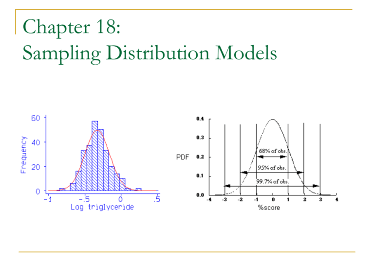
Chapter 18:
Sampling Distribution Models
Modeling the Distribution of
Sample Proportions

Simulate many independent random samples
of equal size


Keep the same probability of success
Histogram of the proportions of the simulated
samples:



Unimodal
Symetric
Centered at p
Normal Model


The center of the histogram is naturally at p, so the
mean of the normal,  is at p.
Once we know p, we automatically know the
standard deviation.
pq
 p 
 Standard deviation:
n
 

Therefore, model the distribution of the sample
proportions with a probability model that is

N  p,


pq 
 ; remember q  1  p
n 
Because we have a normal curve, we can use the
68-95-99.7 Rule.
Assumptions and Conditions

Assumptions



The sampled values must be independent of each
other.
The sample size, n, must be large enough.
Conditions


10% condition: if the sampling has not been made
with replacement, then the sample size, n, must
be no larger than 10% of the population.
Success/Failure condition: The sample size has to
be big enough that both np and nq are greater
than 10.
The Sampling Distribution Model
for a Proportion

In other words, provided that the sampled values are
independent and the sample size is large enough, the
sampling distribution of p is modeled by a Normal
model with mean
 
 
 p  p, and the standard deviation SD p 
z
p p
 
SD p
pq
n
Means


A sample mean also has a sampling
distribution
Simulation: (pp. 353 – 354)




Toss a pair of dice 10,000 times, take the
average, and plot the histogram of the average.
Now toss three die, take the average, and plot the
histogram of the average.
Now toss five die, take the average, and plot the
histogram of the average.
What is happening to the shape of the
histogram?
The Fundamental Theorem of Statistics

Central Limit Theorem:

The sampling distribution model of the sample
mean (and proportion) is approximately Normal
for large n, regardless of the distribution of the
population, as long as the observations are
independent.

The Central Limit Theorem (CLT) talks about the
means of different samples drawn from the same
population, called a sampling distribution model.
Central Limit Theorem

As the sample size, n, increases, the mean of n
independent values has a sampling distribution
that tends towards a Normal model with
 
mean  y equal to the population mean,  ,
 
 
and standard deviation  y  SD y 
z
y
 
SD y

n
.
Assumptions and Conditions


Random sampling condition: the values must
be sampled randomly or the concept of a
sampling distribution makes no sense.
Independence assumption: the sampled
values must be mutually independent. When
the sample is drawn without replacement,
use the

10% condition: the sample size, n, is no more
than 10% of the population.
Law of Diminishing Returns

The standard deviation of the sampling
distribution declines only with the square root
of the sample size.

The square root limits how much we can
make a sample tell about the population.
Standard Error

Often we only know the observed proportion p or
the sample standard deviation, s.

Whenever we estimate the standard deviation of a
sampling distribution, we call it a standard error.


For a proportion, the standard error of p is
For a sample mean, the standard error is
 
SE p 
 
s
SE y 
n
pq
n
WATCH OUT!!

Beware of observations that are not
independent.

Look out for small samples from skewed
populations.

Don’t confuse the sampling distribution with
the distribution of the sample.