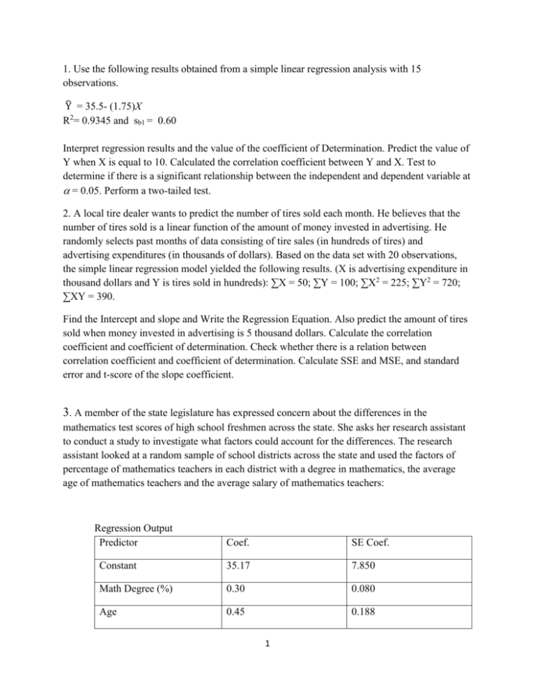
1. Use the following results obtained from a simple linear regression analysis with 15
observations.
̂
Y = 35.5- (1.75)X
R2= 0.9345 and sb1 = 0.60
Interpret regression results and the value of the coefficient of Determination. Predict the value of
Y when X is equal to 10. Calculated the correlation coefficient between Y and X. Test to
determine if there is a significant relationship between the independent and dependent variable at
 = 0.05. Perform a two-tailed test.
2. A local tire dealer wants to predict the number of tires sold each month. He believes that the
number of tires sold is a linear function of the amount of money invested in advertising. He
randomly selects past months of data consisting of tire sales (in hundreds of tires) and
advertising expenditures (in thousands of dollars). Based on the data set with 20 observations,
the simple linear regression model yielded the following results. (X is advertising expenditure in
thousand dollars and Y is tires sold in hundreds): ∑X = 50; ∑Y = 100; ∑X2 = 225; ∑Y2 = 720;
∑XY = 390.
Find the Intercept and slope and Write the Regression Equation. Also predict the amount of tires
sold when money invested in advertising is 5 thousand dollars. Calculate the correlation
coefficient and coefficient of determination. Check whether there is a relation between
correlation coefficient and coefficient of determination. Calculate SSE and MSE, and standard
error and t-score of the slope coefficient.
3. A member of the state legislature has expressed concern about the differences in the
mathematics test scores of high school freshmen across the state. She asks her research assistant
to conduct a study to investigate what factors could account for the differences. The research
assistant looked at a random sample of school districts across the state and used the factors of
percentage of mathematics teachers in each district with a degree in mathematics, the average
age of mathematics teachers and the average salary of mathematics teachers:
Regression Output
Predictor
Coef.
SE Coef.
Constant
35.17
7.850
Math Degree (%)
0.30
0.080
Age
0.45
0.188
1
Salary
0.15
0.075
DF
SS
Regression
3
1120.5
Residual Error
28
530.8
Analysis of Variance
Source
Write the least squares prediction equation. What is the number of observations in the
sample? Based on the multiple regression model given above, estimate the mathematics test
score and calculate the value of the residual, if the percentage of teachers with a mathematics
degree is 50.0, the average age is 45 and the average salary is $48,000. If the actual mathematics
test score for these factors is 68.50, what is the error for this observation? What is the total sum
of squares? What is the explained variation? What is the mean square error and the standard
error of estimate?
4. For the results given in question # 3 above, calculate the Coefficient of Determination and the
Adjusted coefficient of Determination and Test for the overall usefulness of the model using FStatistic at 5% and 1% significance levels. Finally, test the usefulness (or significance of the
three independent variables using t-test for 5% and 1% significance levels.
5. The following table gives the data for per capita income in thousands of US dollars with the
percentage of the labor force in Agriculture and the average years of schooling of the population
over 25 years of age for 15 developed countries in 2000 (data modified for educational purpose).
Develop a multiple regression model for per capita income (dependent variable) using Excel or
MegaStat and answer the questions below the table. You can use symbols Y, X1 and X2 for the
variables in your calculation. Show your computer output.
Country number per capita
% of labor in
Agriculture
Average years of
schooling
1
20
9
7
2
26
10
12
3
24
8
11
4
21
7
11
5
22
10
12
2
5
42
4
16
7
27
5
11
8
24
5
9
9
28
6
12
10
32
8
14
11
30
7
12
12
40
4
16
13
34
9
14
14
30
5
10
15
35
8
13
Find the Y-intercept and slopes for the two independent variables and interpret them. Predict the
per capita income when percentage of labor force in Agriculture is only 3 and average years of
schooling is 15. Find the overall explanatory power (Coefficient of Determination) of the model
and interpret it. Also find the adjusted coefficient of Determination and interpret it. Find the
standard error of estimate. From the ANOVA table find SSR, SSE and SST and the F-value.
Perform the F-test and comment on the overall usefulness of the model Perform t-test for the
statistical significance of individual coefficients.
3