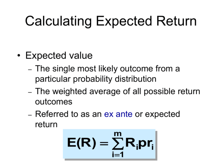
Calculating Expected Return
• Expected value
–
–
–
The single most likely outcome from a
particular probability distribution
The weighted average of all possible return
outcomes
Referred to as an ex ante or expected
return
m
E(R )   Ripri
i1
Calculating Risk
• Variance and standard deviation used to
quantify and measure risk
–
–
–
–
Measures the spread in the probability
distribution
Variance of returns: 2 = (Ri - E(R))2pri
Standard deviation of returns:
 =(2)1/2
Ex ante rather than ex post  relevant
Risk and Return for a portfolio
Two-asset portfolio:
Asset A Asset B
Ri
Ri
Pi
-.05
.25
.30
.10
.10
.40
.25
-.05
.30
E(Ri) .10
.10

.1161895 .1161895
Risk and Return for a portfolio
Wi = % of money invested in asset i.
WA = .5 WB = .5
Pi
-.05 X.5 + .25 X .5 = .10
.30
.10 X .5 + .10 X .5 = .10
.40
.25 X .5 + -.05 X .5 = .10
.30
E(Rp) = .10
p = 0
Covariance
m
COV AB   [ RA,i  E ( RA )][ RB ,i  E ( RB )] pi
i 1
Covariance
COVAB =(-.05 - .10)(.25 - .10)(.30)+
(.10 - .10)(.10 - .10)(.40) +
(.25 - .10)(-.05 - .10)(.30) = -.0135
Assets A and b are negatively covary.
Correlation Coefficient
 AB   AB  A  B
 AB  .0135 / .1161895 x.1161895  1
Correlation Coefficient
Statistical measure of relative comovements between security returns
AB = correlation coefficient between
securities m and n
AB = +1.0 = perfect positive correlation
AB = -1.0 = perfect negative (inverse)
correlation
AB = 0.0 = zero correlation
Portfolio Expected Return
• Weighted average of the individual
security expected returns
–
–
Each portfolio asset has a weight, w,
which represents the percent of the total
portfolio value
The expected return on any portfolio can
be calculated as:
n
E(Rp )   w iE(Ri )
i1
Portfolio Expected Return
WA = .5 and WB =.5
E(Rp) = (.5)(.1) + (.5)(.10) = .10
Portfolio Risk
• Measured by the variance or standard
deviation of the portfolio’s return
–
Portfolio risk is not a weighted average of
the risk of the individual securities in the
portfolio
2 nw 2

p
i
i 1 i


Risk Reduction in Portfolios
• Assume all risk sources for a portfolio of
securities are independent
• The larger the number of securities, the
smaller the exposure to any particular
risk
–
“Insurance principle”
• Only issue is how many securities to
hold
Risk Reduction in Portfolios
• Random diversification
–
–
Diversifying without looking at relevant
investment characteristics
Marginal risk reduction gets smaller and
smaller as more securities are added
• A large number of securities is not
required for significant risk reduction
• International diversification is beneficial
Portfolio Risk and Diversification
p %
Total Portfolio Risk
35
20
Market Risk
0
10
20
30
40
......
Number of securities in portfolio
100+
Random Diversification
• Act of randomly diversifying without
regard to relevant investment
characteristics
• 15 or 20 stocks provide adequate
diversification
Calculating Portfolio Risk
• Two-Security Case:
 p  (w   w   2wA wBCovAB )
2
A
2
A
2
B
2
B
1/ 2
• N-Security Case:
n
n
n
  ( w    wi w j ij ) (i  j )
P
i 1
2
i
2
i
1/ 2
i 1 j 1
Calculating Portfolio Risk
σp =[(.5)2(.1161895)2 +(.5)2(.1161895)2
+2(.5)(.5)(-.0135)]1/2 = 0
The Single-Index Model
 measures the sensitivity of a stock to stock
–
market movements
If securities are only related in their common
response to the market
•
•
Securities covary together only because of their
common relationship to the market index
Security covariances depend only on market risk
and can be written as:
 ij  i  j
2
M