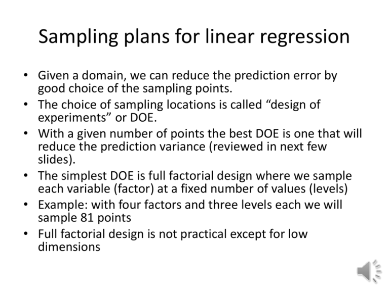
Sampling plans for linear regression
• Given a domain, we can reduce the prediction error by
good choice of the sampling points.
• The choice of sampling locations is called “design of
experiments” or DOE.
• With a given number of points the best DOE is one that will
reduce the prediction variance (reviewed in next few
slides).
• The simplest DOE is full factorial design where we sample
each variable (factor) at a fixed number of values (levels)
• Example: with four factors and three levels each we will
sample 81 points
• Full factorial design is not practical except for low
dimensions
Linear Regression
• Surrogate is linear
n
combination of 𝑛𝑏
yˆ   bii (x)
given shape functions
i 1
• For linear
1  1  2  x
approximation
• Difference (error)
e  y   b  (x ) e  y  Xb
between 𝑛𝑦 data and
surrogate
T
T
e
e

(
y

X
b
)
(y  Xb)
• Minimize square error
• Differentiate to obtain X T Xb  X T y
b
nb
j
j
i 1
i i
j
Model based error for linear
regression
• The common assumptions for linear regression
– The true function is described by the functional form
of the surrogate.
– The data is contaminated with normally distributed
error with the same standard deviation at every point.
– The errors at different points are not correlated.
• Under these assumptions, the noise standard
deviation (called standard error) is estimated as
eT e
ˆ 
n y  nb
2
• 𝜎 is used as estimate of the prediction error.
Prediction variance
n
yˆ   bii (x),
• Linear regression model
i 1
• Define x
(m)
i
 i (x), then
yˆ  x( m)T b,
• With some algebra
Var[ yˆ (x)]  x
( m )T
• Standard error
b x
(m)
( m )T
(m)
X
X
x
  ,
( m )T
X X 
 x
2
s y  ˆ x
T
T
1
1
x( m )
Prediction variance for full factorial design
• Recall that standard error (square root of prediction
1 ( m )
( m )T
T
variance is
s y  ˆ x
X X  x
• For full factorial design the domain is normally a box.
• Cheapest full factorial design: two levels (not good for
quadratic polynomials).
• For a linear polynomial standard error is then
sy 
ˆ
2
n2
1  x12  x22  ....  xn2
• Maximum error at vertices
n 1
s y  ˆ
2n
• What does the ratio in the square root represent?
Quadratic Polynomials
• A quadratic polynomial has (n+1)(n+2)/2 coefficients,
so we need at least that many points.
• Need at least three different values of each variable.
• Simplest DOE is three-level, full factorial design
• Impractical for n>5
• Also unreasonable ratio between number of points and
number of coefficients
• For example, for n=8 we get 6561 samples for 45
coefficients.
• My rule of thumb is that you want twice as many
points as coefficients
Central Composite Design
• Includes 2n vertices, 2n face
points plus nc repetitions of
central point
• Can choose α so to
– achieve spherical design
– achieve rotatibility (prediction
4
variance is spherical) 𝛼 = 𝑉
– Stay in box (face centered) FCCCD
• Still impractical for n>8
Repeated observations at origin
• Unlike linear polynomials, prediction variance
is high at origin.
• Repetition at origin decreases variance there
and improves stability (uniformity).
• Repetition also gives an independent measure
of magnitude of noise.
• Can be used also for lack-of-fit tests.
Without repetition (9 points)
• Contours of
prediction
variance for
spherical CCD
design.
Center repeated 5 times (13 points)
.
• With five repetitions we
reduce the maximum
prediction variance and
greatly improve the
uniformity.
• Five points is the
optimum for uniformity.
D-optimal design
• Maximizes the determinant of XTX to reduce the volume
of uncertainties about the coefficients.
• Example: Given the model y=b1x1+b2x2, and the two data
points (0,0) and (1,0), find the optimum third data point
(p,q) in the unit square.
 0 0
• We have
2


X   1 0


 p q 
1 p
X X 
 pq
T
pq
T
2
det(
X
X
)

q

q2 
• So that the third point is (p,1), for any value of p
• Finding D-optimal design in higher dimensions is a
difficult optimization problem often solved heuristically
Matlab example
1
0.8
>> ny=6;nbeta=6;
>> [dce,x]=cordexch(2,ny,'quadratic');
>> dce'
1 1 -1 -1 0 1
-1 1 1 -1 -1 0
scatter(dce(:,1),dce(:,2),200,'filled')
>> det(x'*x)/ny^nbeta
ans = 0.0055
With 12 points:
>> ny=12;
>> [dce,x]=cordexch(2,ny,'quadratic');
>> dce'
-1 1 -1 0 1 0 1 -1 1 0 -1
1 -1 -1 -1 1 1 -1 -1 0 0 0
scatter(dce(:,1),dce(:,2),200,'filled')
>> det(x'*x)/ny^nbeta
ans =0.0102
0.6
0.4
0.2
0
-0.2
-0.4
-0.6
-0.8
-1
-1
-0.8
-0.6
-0.4
-0.2
0
0.2
0.4
0.6
0.8
1
1
0.8
0.6
0.4
0.2
1
1
0
-0.2
-0.4
-0.6
-0.8
-1
-1
-0.8
-0.6
-0.4
-0.2
0
0.2
0.4
0.6
0.8
1
Problems DOE for regression
• What are the pros and cons of D-optimal
designs compared to central composite
designs?
• For a square, use Matlab to find and plot the
D-optimal designs with 10, 15, and 20 points.
Space-Filling DOEs
• Design of experiments (DOE) for noisy data tend to
place points on the boundary of the domain.
• When the error in the surrogate is due to unknown
functional form, space filling designs are more
popular.
• These designs use values of variables inside range
instead of at boundaries
• Latin hypercubes uses as many levels as points
• Space-filling term is appropriate only for low
dimensional spaces.
• For 10 dimensional space, need 1024 points to have
one per orthant.
Monte Carlo sampling
• Regular, grid-like DOE runs the risk of deceptively
accurate fit, so randomness appeals.
• Given a region in design space, we can assign a
uniform distribution to the region and sample points
to generate DOE.
• It is likely, though, that some regions will be poorly
sampled
• In 5-dimensional space, with 32 sample points, what is
the chance that all orthants will be occupied?
– (31/32)(30/32)…(1/32)=1.8e-13.
Example of MC sampling
1
3
0.8
2
0.6
0.4
1
0.2
0
0
0.5
1
0
0
0.5
1
6
• With 20 points there is evidence
of both clamping and holes
• The histogram of x1 (left) and x2
(above) are not that good either.
4
2
0
0
0.5
1
Latin Hypercube sampling
• Each variable range divided into ny equal probability
intervals. One point at each interval.
1
2
2
3
3
4
4
1
5
5
Latin Hypercube definition matrix
• For n points with m variables: m by n matrix, with
each column a permutation of 1,…,n
• Examples
1 2 4 
1 3
2 1


 3 2 
4 1 2


3 3 3


2 4 1
• Points are better distributed for each variable, but
can still have holes in m-dimensional space.
Improved LHS
• Since some LHS designs are better than others, it is possible to try many
permutations. What criterion to use for choice?
• One popular criterion is minimum distance between points (maximize).
Another is correlation between variables (minimize).
1
• Matlab lhsdesign uses by default 5
iterations to look for “best” design.
• The blue circles were obtained
with the minimum distance
criterion. Correlation coefficient is
-0.7.
• The red crosses were obtained
with correlation criterion, the
coefficient is -0.055.
0.9
0.8
0.7
0.6
0.5
0.4
0.3
0.2
0.1
0
0
0.1
0.2
0.3
0.4
0.5
0.6
0.7
0.8
0.9
1
More iterations
• With 5,000 iterations the two sets of designs improve.
• The blue circles, maximizing minimum distance, still have a correlation
coefficient of 0.236 compared to 0.042 for the red crosses.
1
0.9
• With more iterations,
maximizing the
minimum distance also
reduces the size of the
holes better.
• Note the large holes for
the crosses around
(0.45,0.75) and around
the two left corners.
0.8
0.7
0.6
0.5
0.4
0.3
0.2
0.1
0
0
0.1
0.2
0.3
0.4
0.5
0.6
0.7
0.8
0.9
1
Reducing randomness further
• We can reduce
randomness further by
putting the point at the
center of the box.
• Typical results are
shown in the figure.
• With 10 points, all will
be at 0.05, 0.15, 0.25,
and so on.
1
0.9
0.8
0.7
0.6
0.5
0.4
0.3
0.2
0.1
0
0
0.1
0.2
0.3
0.4
0.5
0.6
0.7
0.8
0.9
1
Problems LHS designs
• Using 20 points in a square, generate a
maximum-minimum distance LHS design, and
compares its appearance to a D-optimal
design.
• Compare their maximum minimum distance
and their det(XTX)