Appendices
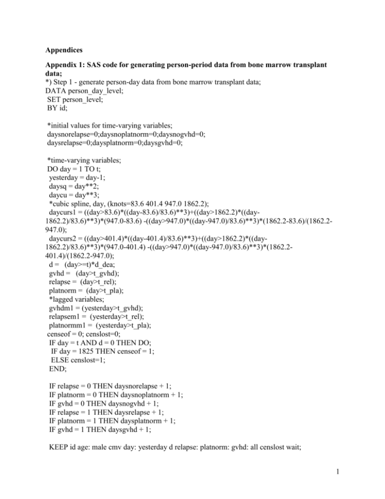
Appendix 1: SAS code for generating person-period data from bone marrow transplant
data;
*) Step 1 - generate person-day data from bone marrow transplant data;
DATA person_day_level;
SET person_level;
BY id;
*initial values for time-varying variables;
daysnorelapse=0;daysnoplatnorm=0;daysnogvhd=0;
daysrelapse=0;daysplatnorm=0;daysgvhd=0;
*time-varying variables;
DO day = 1 TO t;
yesterday = day-1;
daysq = day**2;
daycu = day**3;
*cubic spline, day, (knots=83.6 401.4 947.0 1862.2);
daycurs1 = ((day>83.6)*((day-83.6)/83.6)**3)+((day>1862.2)*((day1862.2)/83.6)**3)*(947.0-83.6) -((day>947.0)*((day-947.0)/83.6)**3)*(1862.2-83.6)/(1862.2947.0);
daycurs2 = ((day>401.4)*((day-401.4)/83.6)**3)+((day>1862.2)*((day1862.2)/83.6)**3)*(947.0-401.4) -((day>947.0)*((day-947.0)/83.6)**3)*(1862.2401.4)/(1862.2-947.0);
d = (day>=t)*d_dea;
gvhd = (day>t_gvhd);
relapse = (day>t_rel);
platnorm = (day>t_pla);
*lagged variables;
gvhdm1 = (yesterday>t_gvhd);
relapsem1 = (yesterday>t_rel);
platnormm1 = (yesterday>t_pla);
censeof = 0; censlost=0;
IF day = t AND d = 0 THEN DO;
IF day = 1825 THEN censeof = 1;
ELSE censlost=1;
END;
IF relapse = 0 THEN daysnorelapse + 1;
IF platnorm = 0 THEN daysnoplatnorm + 1;
IF gvhd = 0 THEN daysnogvhd + 1;
IF relapse = 1 THEN daysrelapse + 1;
IF platnorm = 1 THEN daysplatnorm + 1;
IF gvhd = 1 THEN daysgvhd + 1;
KEEP id age: male cmv day: yesterday d relapse: platnorm: gvhd: all censlost wait;
1
OUTPUT;
END;
RUN;
Appendix 2: SAS code for generating model coefficients for use in G-formula (model
coefficient values given in appendix 6)
*Step 2) - estimate modeling coefficients used to generate probabilities;
TITLE "Parametric G-formula coefficient estimation models";
PROC LOGISTIC DATA = person_day_level DESC;
TITLE2 "Model for probability of relapse=1 at day k";
WHERE relapsem1=0;
MODEL relapse = all cmv male age gvhdm1 daysgvhd platnormm1 daysnoplatnorm agecurs1
agecurs2 day
daysq wait;
ODS OUTPUT ParameterEstimates=rmod(KEEP=variable estimate);*keep model coefficients;
PROC LOGISTIC DATA = person_day_level DESC;
TITLE2 "Model for probability of platnorm=1 at day k";
WHERE platnormm1=0;
MODEL platnorm = all cmv male age agecurs1 agecurs2 gvhdm1 daysgvhd daysnorelapse wait;
ODS OUTPUT ParameterEstimates=Pmod(KEEP=variable estimate);*keep model coefficients;
PROC LOGISTIC DATA = person_day_level DESC;
TITLE2 "Model for probability of exposure=1 at day k";
WHERE gvhdm1=0;
MODEL gvhd = all cmv male age platnormm1 daysnoplatnorm relapsem1 daysnorelapse
agecurs1 agecurs2
day daysq wait;
ODS OUTPUT ParameterEstimates=gmod(KEEP=variable estimate);*keep model coefficients;
PROC LOGISTIC DATA = person_day_level DESC;
TITLE2 "Model for probability of censoring=1 at day k";
MODEL censlost = all cmv male age daysgvhd daysnoplatnorm daysnorelapse agesq day
daycurs1 daycurs2
wait;
ODS OUTPUT ParameterEstimates=cmod(KEEP=variable estimate); *keep model coefficients;
PROC LOGISTIC DATA = person_day_level DESC;
TITLE2 "Model for probability of outcome=1 at day k";
MODEL d = all cmv male age gvhd platnorm daysnoplatnorm relapse daysnorelapse agesq day
daycurs1
daycurs2 wait day*gvhd daycurs1*gvhd daycurs2*gvhd ;
ODS OUTPUT ParameterEstimates=dmod(KEEP=variable estimate);*keep model coefficients;
RUN;
*create data sets with coefficients with prefixes p(platnorm) r(relapse) g(gvhd) c(censoring)
d(death);
DATA Pmod(DROP=i j variable estimate);
SET Pmod END=eof;
j+1;
2
ARRAY p[11];
RETAIN p:;
DO i= 1 TO j; IF i = j THEN p[i] = estimate; END;
IF eof THEN OUTPUT;
DATA Rmod(DROP=i j variable estimate);
SET Rmod END=eof;
j+1;
ARRAY r[14];
RETAIN r:;
DO i= 1 TO j; IF i = j THEN r[i] = estimate; END;
IF eof THEN OUTPUT;
DATA Gmod(DROP=i j variable estimate);
SET Gmod END=eof;
j+1;
ARRAY g[14];
RETAIN g:;
DO i= 1 TO j; IF i = j THEN g[i] = estimate; END;
IF eof THEN OUTPUT;
DATA Cmod(DROP=i j variable estimate);
SET Cmod END=eof;
j+1;
ARRAY c[13];
RETAIN c:;
DO i= 1 TO j; IF i = j THEN c[i] = estimate; END;
IF eof THEN OUTPUT;
DATA Dmod(DROP=i j variable estimate);
SET Dmod END=eof;
j+1;
ARRAY d[18];
RETAIN d:;
DO i= 1 TO j;IF i = j THEN d[i] = estimate; END;
IF eof THEN OUTPUT;
RUN;
*merge model coefficient values into PERSON LEVEL data;
DATA person_level_w_coefs;
SET person_level;
IF _N_=1 THEN DO;
SET pmod;
SET gmod;
SET rmod;
SET dmod;
SET cmod;
END;
RUN;
3
Appendix 3: Drawing Monte Carlo sample and running natural course / GvHD
intervention using G-formula
*Step 3) - sample with replacement from data;
PROC SURVEYSELECT DATA=person_level_w_coefs SEED=12131231 OUT=mcsample
METHOD=URS N=137000 OUTHITS;
RUN;
*Step 4 and 5) - run Monte Carlo sample for natural course, always and never GvHD;
DATA natcourse(KEEP = id all cmv male age d td gvhd tg platnorm tp relapse tr)
alwaysgvhd(KEEP = id all cmv male age d td gvhd tg platnorm tp relapse tr)
nevergvhd(KEEP = id all cmv male age d td gvhd tg platnorm tp relapse tr);
SET mcsample; *set each time the intervention changes;
BY id;
CALL STREAMINIT(187100);
DO intervention = 0 TO 2;
* RETAIN done 0;
day = 0;
done = 0;
DO WHILE (day <= 1825 AND done=0);
day+1;
daysq = day**2;
daycu = day**3;
*cubic spline, day, (knots=83.6 401.4 947.0 1862.2);
daycurs1 = ((day>83.6)*((day-83.6)/83.6)**3)+((day>1862.2)*((day1862.2)/83.6)**3)*(947.0-83.6) -((day>947.0)*((day-947.0)/83.6)**3)*(1862.2-83.6)/(1862.2947.0);
daycurs2 = ((day>401.4)*((day-401.4)/83.6)**3)+((day>1862.2)*((day1862.2)/83.6)**3)*(947.0-401.4) -((day>947.0)*((day-947.0)/83.6)**3)*(1862.2401.4)/(1862.2-947.0);
IF day =1 THEN DO; *set baseline variables;
relapse=0;gvhd=0;platnorm=0;
gvhdm1=0;relapsem1=0;platnormm1=0;
daysnorelapse=0;daysnoplatnorm=0;daysnogvhd=0;
daysrelapse=0;daysplatnorm=0;daysgvhd=0;
END;*set baseline variables;
ELSE DO;*set time-varying variables - lag is built in;
IF relapse = 0 THEN daysnorelapse + 1;
ELSE daysrelapse + 1;
IF platnorm = 0 THEN daysnoplatnorm + 1;
ELSE daysplatnorm + 1;
IF gvhd = 0 THEN daysnogvhd + 1;
ELSE daysgvhd + 1;
*platelets (Time-varying covariate L1);
IF platnormm1=1 THEN platnorm=1; *assume platelets stay normal once they reach normal
levels;
ELSE DO; *normal platelet probability at day k;
4
logitpp = p1 + p2*all + p3*cmv + p4*male + p5*age + p6*agecurs1 + p7*agecurs2 +
p8*gvhdm1 + p9*daysgvhd + p10*daysnorelapse + p11*wait;
IF logitpp <-700 THEN gvhd = 1;*avoid machine error;
ELSE platnorm=RAND("bernoulli",1/(1+exp(-(logitpp))));
END; *normal platelet probability at day k;
*relapse(Time-varying covariate L2);
IF relapsem1=1 THEN relapse=1; *assume relapse is not cured once patient experiences first
post transplant relapse;
ELSE DO; *relapse probability at day k;
logitpr= r1 + r2*all + r3*cmv + r4*male + r5*age + r6*gvhdm1 + r7*daysgvhd +
r8*platnormm1 + r9*daysnoplatnorm + r10*agecurs1 + r11*agecurs2 + r12*day + r13*daysq +
r14*wait;
IF logitpr <-700 THEN relapse = 1; *avoid machine error;
ELSE relapse=RAND("bernoulli",1/(1+exp(-(logitpr))));
END;*relapse probability at day k;
END;
*GvHD (main exposure A);
IF gvhdm1=1 THEN gvhd=1; *assume patients can't be cured of GvHD once GvHD onset
occurs;
ELSE DO; *gvhd onset probability at day k;
logitpg = g1 + g2*all + g3*cmv + g4*male + g5*age + g6*platnormm1 + g7*daysnoplatnorm
+ g8*relapsem1 + g9*daysnorelapse + g10*agecurs1 + g11*agecurs2 + g12*day + g13*daysq +
g14*wait;
IF logitpG <-700 THEN gvhd = 1; *avoid machine error;
ELSE gvhd = RAND("bernoulli",1/(1+exp(-(logitpg))));
END;*gvhd onset probability at day k;
*intervene on exposure;
IF intervention = 0 THEN gvhd=gvhd; *natural course;
ELSE IF intervention = 1 THEN gvhd=1; *always GvHD;
ELSE IF intervention = 2 THEN gvhd=0; *never GvHD;
IF done=0 THEN DO; *censoring and death probability at day k;
*censoring probability at day k;
logitpc = c1 + c2*all + c3*cmv + c4*male + c5*age + c6*daysgvhd + c7*daysnoplatnorm +
c8*daysnorelapse + c9*agesq + c10*day + c11*daycurs1 + c12*daycurs2 + c13*wait;
IF logitpc <-700 THEN d = 1; *avoid machine error;
ELSE cens = RAND("bernoulli",1/(1+exp(-(logitpc))));
IF intervention > 0 THEN cens=0; *intervening to prevent censoring for everything but
natural course;
done=cens;
IF done=0 THEN DO; *if not censored on day k;
*death probability at day k;
logitpd = d1 + d2*all + d3*cmv + d4*male + d5*age + d6*gvhd + d7*platnorm +
d8*daysnoplatnorm + d9*relapse + d10*daysnorelapse + d11*agesq + d12*day + d13*daycurs1
+ d14*daycurs2 + d15*wait + d16*day*gvhd + d17*daycurs1*gvhd + d18*daycurs2*gvhd;
5
IF logitpd <-700 THEN d = 1;*avoid machine error;
ELSE d = RAND("bernoulli",1/(1+exp(-(logitpd))));
done=d;
END;*if not censored on day k;
IF day >= 1825 THEN done=1;
IF gvhd=1 AND gvhdm1=0 THEN tg=day;
IF relapse=1 AND relapsem1=0 THEN tr = day;
IF platnorm=1 AND platnormm1=0 THEN tp = day;
IF done=1 THEN DO;
td=day;
IF gvhd=0 THEN tg=day+1;
IF relapse=0 THEN tr=day+1;
IF platnorm=0 THEN tp=day+1;
IF intervention = 0 THEN OUTPUT natcourse; *output a PERSON LEVEL dataset;
ELSE IF intervention = 1 THEN OUTPUT alwaysgvhd; *output a PERSON LEVEL dataset
if intervention is always GvHD;
ELSE IF intervention = 2 THEN OUTPUT nevergvhd; *output a PERSON LEVEL dataset if
intervention is never GvHD;
END;*censoring and death probability at day k;
END;*set time-varying variables;
*lagged variables;
relapsem1=relapse;
platnormm1=platnorm;
gvhdm1=gvhd;
END; * while done = 0 and day < 1825;
END;*intervetion from 0 to 2;
RUN;
*Step 6) concatentate intervetion data sets and run Cox model;
DATA gformula;
SET alwaysgvhd nevergvhd;
PROC PHREG DATA = gformula;
MODEL td*d(0) = gvhd / TIES=EFRON RL;
RUN;
PROC PHREG DATA = gformula;
MODEL td*d(0) = gvhd1 gvhd2 / TIES=EFRON RL;
gvhd1=gvhd*(td<=100); gvhd2=gvhd*(td>100);
RUN;
Appendix 4: SAS code to read bone marrow transplant data;
DATA person_level;
INPUT id t t_rel d_dea t_gvhd d_gvhd d_rel t_pla d_pla age male cmv waitdays all ;
6
DATALINES;
1 1 1 1 1 0 0 1 0 42 1 0 196 1
2 2 2 1 2 0 0 2 0 20 1 0 75 0
3 10 10 1 10 0 0 10 0 34 1 1 240 0
4 16 16 1 16 0 0 16 0 27 0 1 180 0
5 35 35 1 35 0 0 35 0 23 0 1 150 0
6 48 48 1 48 0 0 14 1 32 0 1 150 0
7 53 53 1 53 0 0 53 0 33 0 1 180 0
8 62 47 1 62 0 1 11 1 27 1 0 90 0
9 63 63 1 38 1 0 16 1 44 1 0 360 0
10 73 64 1 73 0 1 38 1 45 0 1 180 0
11 74 74 1 29 1 0 24 1 41 0 1 750 0
12 79 79 1 16 1 0 79 0 43 0 0 90 0
13 80 80 1 10 1 0 80 0 30 0 0 150 0
14 80 80 1 21 1 0 0 1 35 1 0 780 0
15 86 86 1 86 0 0 86 0 17 1 1 239 1
16 93 47 1 93 0 1 28 1 7 1 0 135 0
17 97 76 1 97 0 1 97 0 48 1 1 330 0
18 105 105 1 21 1 0 15 1 37 1 1 120 0
19 105 105 1 105 0 0 105 0 14 1 0 150 0
20 105 48 1 105 0 1 30 1 17 0 0 210 0
21 107 107 1 107 0 0 107 0 30 1 1 178 1
22 110 74 1 110 0 1 49 1 28 1 1 303 1
23 121 100 1 28 1 1 65 1 39 1 1 210 0
24 122 122 1 88 1 0 13 1 20 1 0 2616 1
25 122 120 1 122 0 1 12 1 25 0 1 510 0
26 128 115 1 128 0 1 12 1 37 0 1 270 0
27 129 93 1 129 0 1 51 1 37 0 1 240 0
28 153 113 1 153 0 1 59 1 31 0 1 240 0
29 156 104 1 28 1 1 20 1 20 1 0 85 1
30 162 109 1 162 0 1 40 1 36 1 1 393 1
31 162 162 1 162 0 0 13 1 22 1 0 300 0
32 164 164 1 164 0 0 164 0 19 0 0 285 0
33 168 168 1 168 1 0 48 1 32 0 1 150 0
34 172 172 1 22 1 0 37 1 40 0 0 129 1
35 183 183 1 130 1 0 21 1 11 0 0 120 0
36 194 194 1 94 1 0 25 1 26 0 0 329 1
37 195 32 1 195 0 1 16 1 36 1 0 90 0
38 222 219 1 123 1 1 52 1 28 1 1 120 0
39 226 226 0 226 0 0 10 1 18 0 0 208 1
40 243 122 1 243 0 1 23 1 37 0 1 170 1
41 248 157 1 100 1 1 52 1 33 0 1 180 0
42 262 192 1 10 1 1 59 1 29 1 1 74 1
43 262 55 1 262 0 1 24 1 23 0 1 331 1
44 265 242 1 210 1 1 14 1 32 1 0 180 0
45 269 110 1 120 1 1 27 1 29 0 1 361 1
7
46 276 276 1 81 1 0 21 1 18 0 0 146 1
47 288 288 1 18 1 0 288 0 45 1 1 90 0
48 318 318 1 140 1 0 12 1 35 0 1 300 0
49 341 268 1 21 1 1 17 1 20 0 1 180 0
50 350 332 1 350 0 0 33 1 22 1 0 834 1
51 363 363 1 363 0 0 19 1 52 1 1 180 0
52 371 230 1 184 1 1 9 1 39 0 0 147 1
53 390 390 1 390 0 0 11 1 50 1 0 120 0
54 392 273 1 122 1 1 24 1 43 1 1 240 0
55 393 381 1 100 1 1 16 1 33 0 0 120 0
56 414 414 1 414 0 0 27 1 21 1 0 120 0
57 417 383 1 417 0 1 16 1 15 1 0 824 1
58 418 418 1 220 1 0 21 1 18 1 0 110 1
59 431 272 1 431 0 1 12 1 30 0 1 120 0
60 466 466 1 119 1 0 100 1 15 1 0 508 1
61 469 467 1 90 1 1 20 1 35 0 1 120 0
62 481 481 1 30 1 0 24 1 35 1 1 90 0
63 487 487 1 76 1 0 22 1 22 1 0 128 1
64 491 422 1 180 1 1 491 0 22 0 0 210 0
65 515 390 1 515 0 1 31 1 23 1 1 210 0
66 522 421 1 25 1 1 20 1 28 1 0 90 0
67 526 526 1 121 1 0 11 1 15 1 0 943 1
68 530 530 0 38 1 0 34 1 17 1 0 151 1
69 547 456 1 130 1 1 24 1 31 1 1 630 0
70 583 486 1 583 0 1 11 1 17 0 0 120 0
71 641 641 1 641 0 0 11 1 26 1 0 90 0
72 653 211 1 653 0 1 23 1 23 1 0 90 0
73 677 677 1 150 1 0 8 1 15 1 1 150 0
74 704 704 1 36 1 0 18 1 29 0 1 105 0
75 716 662 1 716 0 1 17 1 28 1 0 84 1
76 732 625 1 732 0 1 18 1 39 0 1 150 0
77 781 609 1 781 0 1 26 1 27 1 1 187 1
78 845 845 0 845 0 0 20 1 40 0 1 210 0
79 847 847 0 847 0 0 16 1 28 1 0 75 0
80 848 848 0 155 1 0 16 1 23 1 0 180 0
81 860 860 0 860 0 0 15 1 25 0 0 180 0
82 932 932 0 29 1 0 7 1 27 0 0 60 0
83 957 957 0 957 0 0 69 1 18 1 0 90 0
84 996 996 0 72 1 0 12 1 22 1 0 1319 1
85 1030 1030 0 210 1 0 14 1 25 0 0 210 0
86 1063 1063 1 240 1 0 16 1 50 1 1 270 0
87 1074 1074 1 120 1 0 19 1 30 1 1 150 0
88 1111 1111 0 1111 0 0 22 1 19 1 0 236 1
89 1136 1136 0 140 1 0 15 1 47 1 1 900 0
90 1156 748 1 180 1 1 18 1 14 1 0 60 0
91 1167 1167 0 39 1 0 1167 0 27 0 1 191 1
8
92 1182 1182 0 112 1 0 22 1 24 0 0 203 1
93 1199 1199 0 91 1 0 29 1 24 1 0 174 1
94 1238 1238 0 250 1 0 18 1 24 1 1 240 0
95 1258 1258 0 120 1 0 66 1 30 0 1 180 0
96 1279 129 1 1279 0 1 22 1 17 0 0 937 1
97 1298 84 1 1298 0 1 1298 0 8 0 1 105 0
98 1324 1324 0 25 1 0 15 1 46 1 1 75 0
99 1330 1330 0 96 1 0 17 1 20 1 1 1006 1
100 1345 1345 0 32 1 0 14 1 50 1 1 120 0
101 1356 606 0 1356 0 1 14 1 33 1 1 210 0
102 1363 1363 0 200 1 0 12 1 13 1 1 90 0
103 1377 1377 0 123 1 0 12 1 22 1 1 2187 1
104 1384 1384 0 200 1 0 19 1 21 0 0 120 0
105 1433 1433 0 236 1 0 12 1 32 1 1 93 1
106 1447 1447 0 220 1 0 24 1 33 0 1 150 0
107 1462 1462 0 70 1 0 13 1 17 0 0 168 1
108 1470 1470 0 180 1 0 14 1 27 1 0 240 0
109 1496 1496 0 307 1 0 12 1 26 1 1 127 1
110 1499 248 0 1499 0 1 9 1 35 1 0 30 0
111 1527 1527 0 1527 0 0 13 1 22 0 0 450 0
112 1535 1535 0 1535 0 0 21 1 35 0 0 180 0
113 1562 1562 0 1562 0 0 18 1 26 1 1 90 0
114 1568 1568 0 1568 0 0 14 1 15 1 0 90 0
115 1602 1602 0 139 1 0 18 1 21 1 0 1720 1
116 1631 1631 0 150 1 0 40 1 27 1 1 690 0
117 1674 1674 0 1674 0 0 24 1 37 1 0 60 0
118 1709 1709 0 20 1 0 19 1 23 0 1 90 0
119 1799 1799 0 140 1 0 12 1 32 1 0 120 0
120 1825 1825 0 1825 0 0 19 1 19 1 1 210 0
121 1825 1825 0 1825 0 0 19 1 34 0 1 270 0
122 1825 1825 0 1825 0 0 9 1 37 0 0 180 0
123 1825 1825 0 260 1 0 15 1 29 0 1 90 0
124 1825 1825 0 230 1 0 16 1 33 0 1 225 0
125 1825 1825 0 180 1 0 16 1 35 0 0 105 0
126 1825 1825 0 67 1 0 13 1 26 1 1 98 1
127 1825 1825 0 250 1 0 17 1 36 0 0 240 0
128 1825 1825 0 220 1 0 18 1 27 1 1 210 0
129 1825 1825 0 1825 0 0 12 1 25 0 0 60 0
130 1825 1825 0 1825 0 0 11 1 16 1 1 60 0
131 1825 1825 0 52 1 0 15 1 45 0 0 105 0
132 1825 1825 0 150 1 0 17 1 35 1 0 120 0
133 1825 1825 0 1825 0 0 16 1 35 1 1 120 0
134 1825 1825 0 1825 0 0 14 1 29 1 0 24 0
135 1825 1825 0 1825 0 0 17 1 31 1 0 60 0
136 1825 1825 0 1825 0 0 21 1 19 1 1 270 0
137 1825 1825 0 1825 0 0 22 1 18 1 0 750 0
9
;
*define more baseline covariates;
DATA person_level;
SET person_level;
*baseline variables;
wait = waitdays/30.5;
agesq = age**2;
*restricted cubic spline on age (knots at 17, 25.4, 30, 41.4);
agecurs1 = (age>17.0)*(age-17.0)**3-((age>30.0)*(age-30.0)**3)*(41.4-17.0)/(41.4-30.0);
agecurs2 = (age>25.4)*(age-25.4)**3-((age>41.4)*(age-41.4)**3)*(41.4-25.4)/(41.4-30.0);
RUN;
10
Appendix 5:
Formal treatment of the parametric G-formula
We adopt the “do notation” of Pearl (2009) to express the potential outcomes and
covariate values we would observe under interventions, where, for example 𝑋(𝑑𝑜(𝐵 = 𝑏)) is the
value we would expect X to take on if we could intervene on B by setting it to the value “b” (i.e.
uppercase letters are random variables, and lowercase letters are realizations). While all
covariates are recorded at the individual level, we omit the subscript i for clarity. Bold font is
used to denote vectors. Time is subscripted and history variables are denoted with an overbar,
where a history variable 𝐵̅𝑘 = (𝐵0 , … , 𝐵𝑘 ), is an expanding set of time-specific random variables
or a summary of the history (such as the cumulative time on treatment) through time k. Notation
for our data is shown in Appendix Table 1.
The G-formula for the bone marrow transplant data
Using our data, the G-formula for the marginal incidence of death by the end of follow up
at time j (Ij) under no intervention can be expressed as:
𝐼𝑗
̅ 𝒌 = 𝒍̅𝒌 , 𝑽𝟎 = 𝒗𝟎 , 𝑌𝑘−1 = 0) ×
𝑃𝑟(𝑌𝑘 = 1| 𝐴𝑘 = 𝑎𝑘 , 𝐴̅𝑘 = 𝑎̅𝑘 , 𝑳𝒌 = 𝒍𝒌 , 𝑳
̅ 𝒎 = 𝒍̅𝒎 , 𝑽𝟎 = 𝒗𝟎 , 𝑌𝑚−1 = 𝐶𝑚−1 = 0) ×
𝑃𝑟(𝐶𝑚 = 0| 𝐴𝑚 = 𝑎𝑚 , 𝐴̅𝑚 = 𝑎̅𝑚 , 𝑳𝒎 = 𝒍𝒎 , 𝑳
𝑗
𝑘
̅ 𝒎 = 𝒍̅𝒎 , 𝑽𝟎 = 𝒗𝟎 , 𝑌𝑚−1 = 𝐶𝑚−1 = 0) ×
𝑃𝑟(𝐴𝑚 = 𝑎𝑚 | 𝐴̅𝑚−1 = 𝑎̅𝑚−1 , 𝑳𝒎 = 𝒍𝒎 , 𝑳
= ∑∑∑∑
∏ 𝑃𝑟(𝐿𝑚 = 𝑙𝑚 | 𝐴𝑚−1 = 𝑎𝑚−1 , 𝐴̅𝑚−1 = 𝑎̅𝑚−1 , 𝑳
̅ 𝒎 = 𝒍̅𝒎 , 𝑽𝟎 = 𝒗𝟎 , 𝑌𝑚−1 = 𝐶𝑚−1 = 0) ×
𝑘=1 𝒗
𝑙
𝑎
𝑚=1 𝑃𝑟(𝑉 = 𝑣 ) ×
0
0
̅ 𝒎−𝟏 = 𝒍̅𝒎−𝟏 , 𝑽𝟎 = 𝒗𝟎 , 𝑌𝑚−2 = 𝐶𝑚−2 = 0)]}
[𝑃𝑟 (𝑌𝑚−1 = 0| 𝐴𝑚−1 = 𝑎𝑚−1 , 𝐴̅𝑚−1 = 𝑎̅𝑚−1 , 𝑳𝒎−𝟏 = 𝒍𝒎−𝟏 , 𝑳
{
11
Where time specific conditional probability of Yk at each time point is multiplied by the
conditional probabilities (or probability densities) of Ak,, Lk, and V0 and summed over the
observed values of ak,, lk and v0. Because V0 includes only baseline covariates, it is not assumed
to be a function of any other variables of interest. With enough data and if all variables were low
dimension (e.g. dichotomous), we could identify the time specific probability of each variable in
the set (𝑌𝑘 , 𝐶𝑘 , 𝐴𝑘 , 𝐴̅𝑘−1 , 𝑳𝒌 , 𝑳̅𝒌−𝟏 , 𝑉0 ) simply by taking sample proportions (i.e. the model is nonparametrically identified). However, this cohort is followed for 1825 days and we include
continuous covariates, so we must model each probability.
3. Parametric G-formula algorithm
Step 1) From a one-record-per-person data set recording baseline covariates, and time to:
relapse; normal platelet count; GvHD; and death or censoring, create a person-period data set in
which each record corresponds to one person-day (for example, the third person in the data set
given appendix 4 who survives to day 10 has 10 records in the dataset). Each person-period
record contains a variable k recording the number of days since transplant as well as the set of
variables (𝑌𝑘 , 𝐶𝑘 , 𝐴𝑘 , 𝐴̅𝑘 , 𝑳𝒌 , 𝑳̅𝒌 , 𝑉0 ).
Step 2) Use a pooled logistic model to estimate the conditional probability of each of the
time-varying covariates, including the exposure. When the time-specific conditional probability
of the covariate is low (say Pr(𝑌𝑘 = 1| ⋅) < 0.1), coefficients from a pooled logistic model with
flexible terms for time (e.g., spline) closely approximate those of a Cox model (Abbot 1985). We
used the SAS procedure LOGISTIC to output model coefficients. For our example data, the
12
pooled logistic model to estimate the probability of developing GvHD at time k (the second line
in the G-formula above) was
Pr(𝐴𝑘 = 1| 𝐴̅𝑘−1 = 0, 𝑳𝒌 , 𝑳̅𝒌 , 𝑽𝟎 , 𝑌𝑘−1 = 𝐶𝑘−1 = 0; 𝛼) =
𝑒𝑥𝑝𝑖𝑡(∑𝛼̂𝐺 𝑮𝒌 + ∑𝛼̂𝐿 𝑳𝒌 + ∑𝛼̂𝐿̅ 𝑳̅𝒌 + ∑𝛼̂𝑉 𝑽𝟎 )
and the logistic model for death at time k was
Pr(𝑌𝑘 = 1| 𝐴𝑘 , 𝐴̅𝑘−1 , 𝑳𝒌 , 𝑳̅𝒌 , 𝑽𝟎 , 𝑌𝑘−1 = 𝐶𝑘−1 = 0; 𝜔) =
expit(∑𝜔
̂𝐺 𝑮𝒌 + 𝜔
̂𝐴 𝐴𝑘 + 𝜔
̂𝐴̅ 𝐴̅𝑘−1 + ∑𝜔
̂𝐺𝐴 𝑮𝒌 𝐴𝑘 + ∑𝜔
̂𝐿 𝑳𝒌 + ∑𝜔
̂𝐿̅ 𝑳̅𝒌 + ∑𝜔
̂ 𝑉 𝑽𝟎 )
Where expit(⋅) = exp(⋅)/(1 + exp(⋅)) is the inverse-logit function, 𝑮𝒌 is a vector of
terms representing a restricted cubic spline for days on study (day k) with knots at the 10th, 40th,
60th and 90th percentiles (83, 401, 947 and 1862 days), and the 𝛼̂ (or 𝜔
̂) coefficients represent the
difference in log-odds of GvHD onset (or death) on day k for a one unit difference in each
covariate. The hat accent over the coefficients is to emphasize that we are estimating these
coefficients from the data. The baseline covariates in 𝑽𝟎 , the current and prior time-varying
confounder vectors 𝑳𝒌 and 𝑳̅𝒌 , and current and prior GvHD variables 𝐴𝑘 and 𝐴̅𝑘 are as described
in the notation section, and the summation symbol 𝛴 is used to indicate that each covariate
within a vector will be associated with a unique coefficient. Additionally ∑𝑮𝒌 𝐴𝑘 is set of
product terms between GvHD and the spline variables for time to allow for changing direct
exposure effects over time. Using the terminology of directed acyclic graphs, the set of
covariates (𝐴̅𝑘 , 𝑳𝒌 , 𝑳̅𝒌 , 𝑽𝟎 ) should be a sufficient set of covariates such that conditioning on them
blocks all non-causal pathways from exposure to the outcome (Pearl 2009 Ch 4).
13
Because we are modeling the onset of GvHD, the model for 𝐴𝑘 is conditioned on 𝐴̅𝑘−1 =
0 (the patient is GvHD free up until just before day k) by restricting the logistic model to the
subset of the data where 𝐴̅𝑘−1 = 0. The person-period data contain observations only for the
days from the first day after transplant to the day of death or censoring, so all of our models are
implicitly conditioned on 𝑌𝑘−1 = 𝐶𝑘−1 = 0.
We also used pooled logistic models for 𝑳𝒌 = (𝐿1𝑘 , 𝐿2𝑘 ) where 𝐿1𝑘 is platelet level and
𝐿2𝑘 is relapse, where
Pr(𝐿1𝑘 = 1| 𝐴𝑘−1 , 𝐴̅𝑘−1 , 𝐿̅1𝑘−1 = 0, 𝐿̅2𝑘−1 , 𝑽𝟎 , 𝑌𝑘−1 = 𝐶𝑘−1 = 0; 𝛽) =
𝑒𝑥𝑝𝑖𝑡(∑𝛽̂𝐺 𝑮𝒌 + 𝛽̂𝐴 𝐴𝑘−1 + 𝛽̂𝐴̅ 𝐴̅𝑘−1 + 𝛽̂𝐿̅2 𝐿̅2𝑘−1 + ∑𝛽̂𝑉 𝑽𝟎 )
and
Pr(𝐿2𝑘 = 1|𝐴𝑘−1 , 𝐴̅𝑘−1 , 𝐿1𝑘 , 𝐿̅1𝑘−1 , 𝐿̅2𝑘−1 = 0, 𝑽𝟎 , 𝑌𝑘−1 = 𝐶𝑘−1 = 0; 𝛾) =
𝑒𝑥𝑝𝑖𝑡(∑𝛾̂𝐺 𝑮𝒌 + 𝛾̂𝐴 𝐴𝑘−1 + 𝛾̂𝐴̅ 𝐴̅𝑘−1 + 𝛾̂𝐿1 𝐿𝑘 + 𝛾̂𝐿̅1 𝐿̅1𝑘−1 + ∑𝛾̂𝑉 𝑽𝟎 )
As in the logistic model for GvHD, 𝑮𝒌 is a flexible function of time, 𝑽𝟎 are the baseline
covariates, and we model the return of normal platelet counts or relapse by conditioning on
𝐿̅1𝑘−1 = 0 (or 𝐿̅2𝑘−1 = 0). 𝐿̅1𝑘−1 and 𝐿̅2𝑘−1 are the days spent without normal platelet counts or
without relapsing. The 𝛽̂ (or 𝛾̂) parameters represent the difference in the log odds of return to
normal platelet counts (or relapse) on day k for a one-unit increment of the corresponding
covariate. We assume that, in a given day the temporal order is (𝐿1𝑘 , 𝐿2𝑘 , 𝐴𝑘 , 𝐶𝑘 , 𝑌𝑘 ). The logodds of censoring was assumed to be a linear function of baseline covariates, cumulative days
14
with abnormal platelet counts, cumulative days spent relapse-free, and cumulative days with
GvHD.
Step 3) From our original sample of N=137, we re-sampled with replacement M=137,000
pseudo-patients, retaining only baseline covariates V0. The large sample reduces Monte Carlo
error, and should be as large as is practical. Resampling can be done, for example, using the SAS
procedure SURVEYSELECT.
Step 4) Using model coefficients generated in Step 2 and the baseline covariates from our
137,000 pseudo-patients, we generated follow-up data for each of the M pseudo-patients by
imputing values for platelet levels, relapse, and graph-versus host disease. Time-varying
covariates at baseline were set to A0=0, and L0=(0,0). We also imputed the outcome variable Y1,
using observed baseline covariates and the imputed values for A1 and L1. Similar to the dataset
created in step one, we retained a record for each of the 137,000 pseudo-patients for each personday. For example, the value of 𝐴𝑘 (the indicator of GvHD on day k) for individuals who were
previously GvHD-free and not yet censored or dead was generated from a binomial distribution
with
Pr(𝐴𝑘 = 1| 𝑳𝒌 , 𝑳̅𝒌−𝟏 , 𝑽𝟎 ) =
𝑒𝑥𝑝𝑖𝑡(∑𝛼̂𝐺 𝑮𝒌 + ∑𝛼̂𝐿 𝑳𝒌 + ∑𝛼̂𝐿̅ 𝑳̅𝒌−𝟏 + ∑𝛼̂𝑉 𝑽𝟎 )
Step 2 can be performed in SAS with a single DATA step using DO loops to cycle
through days 1 to 1825 (or until 𝑌𝑘 = 1 or 𝐶𝑘 = 1), and the GvHD values can be imputed for
each person day by drawing a value from a Bernoulli distribution with the probability of GvHD
onset (Pr(𝐴𝑘 = 1| 𝑳𝒌 , 𝑳̅𝒌−𝟏 , 𝑽𝟎 )) given above. As was observed in our example data, we set this
probability to 1 if the pseudo-patient developed GvHD on a previous day.
15
Exposure, covariate, censoring and outcome values for each subsequent day were
imputed in the same way, using imputed covariate values from previous days (e.g. day k-1) to
generate new values for subsequent days. Any pseudo-patient with 𝑌𝑘 = 1 or 𝐶𝑘 = 1 did not
receive subsequent records for times k+1, …, 1825.
Rather than model the distribution of the baseline covariates in 𝑽𝟎 from which we could
have generated baseline covariates values, we used the joint empirical distribution of the baseline
covariates. To do this, we kept the baseline covariate values from our original data (N) and used
them to generate time-varying covariate values for days k > 1 in our pseudo data (M). With this
Monte Carlo dataset we checked marginal survival curves and covariate distributions against
those from the observed data. Model selection was carried out by repeating Steps 1 and 2, and
varying the parametric forms (e.g., … ) of each model until the marginal survival curves and
covariate distributions in the Monte Carlo data (M) closely approximated those in the observed
data (N). We refer to the data M generated from this set of models as the “natural course.”
Step 5) We repeated Step 4 using two interventions: a) “Always GvHD:” set GvHD to 1
on day 1 and impute all other covariates as before, and b) “Never GvHD:” set GvHD to 0 and
impute all other covariates, not allowing GvHD status to change. In both interventions, we set
𝐶𝑘 = 0 for all censoring other than the end of follow up. With no drop out and no competing
risks, we could estimate E[Y(do(Ak =1))] and E[Y(do(Ak =0))] by simply taking sample
proportions of the deaths in each simulated dataset.
For example, the model to impute the return to normal platelet counts for the data for the
intervention 𝑑𝑜(𝐴𝑘 = 1) is expressed as:
Pr(𝐿1𝑘 = 1| 𝐴𝑘−1 , 𝐴̅𝑘−2 , 𝐿̅2𝑘−1 , 𝑽𝟎 ; 𝛽) =
16
𝑒𝑥𝑝𝑖𝑡(∑𝛽̂𝐺 𝑮𝒌 + 𝛽̂𝐴 𝐴𝑘−1 + 𝛽̂𝐴̅ 𝐴̅𝑘−1 + 𝛽̂𝐿̅2 𝐿̅2𝑘−1 + ∑𝛽̂𝑉 𝑽𝟎 ) =
𝑒𝑥𝑝𝑖𝑡(∑𝛽̂𝐺 𝑮𝒌 + 𝛽̂𝐴 1 + 𝛽̂𝐴̅ (𝑘 − 1) + 𝛽̂𝐿̅2 𝐿̅2𝑘−1 + ∑𝛽̂𝑉 𝑽𝟎 )
Where GvHD (𝐴𝑘−1 ) is always 1 and days since onset of GvHD (𝐴̅𝑘−1 ) is the number of
days since transplant. The intervention is carried out across all four models (i.e. the models for
return to normal platelet count, relapse, GvHD, and death) and yields data, the distribution of
which corresponds to what we would observe in the population of bone marrow transplant had
we been able to implement the intervention 𝑑𝑜(𝐴𝑘 = 1) (i.e. give all patients GvHD
immediately after surgery). We repeat this process setting GvHD to 0 for every day k.
Step 6) We concatenated the datasets from step 5 and fit a marginal structural Cox
proportional hazards model to the simulated dataset to estimate the HR comparing the hazard of
Y(do(Ak =1)) to the hazard of Y(do(Ak =0)), which, under assumptions outlined later can be
interpreted as a causal HR. The marginal structural Cox model for the potential failure times
𝑇(𝑑𝑜(𝐴𝑘 = 𝑎)) can be expressed as:
𝜆∗𝑘1 = 𝜆∗𝑘0 (exp(𝜂𝐴𝑘 ))
and, for a = 1 or 0
𝜆∗𝑘𝑎 = lim (
𝛿𝑘→0
Pr(𝑘 < 𝑇(𝑑𝑜(𝐴𝑘 = 𝑎)) < 𝑘 + 𝛿𝑘|𝑇(𝑑𝑜(𝐴𝑘 = 𝑎)) > 𝑘)
)
𝛿𝑘
Where 𝑇(𝑑𝑜(𝐴𝑘 = 𝑎)) is the day on which death occurred and the hazards 𝜆∗𝑘1 and 𝜆∗𝑘0
for the potential outcomes we would observe under the interventions do(Ak =1) and do(Ak =0).
Because the generated data from step 5 correspond to the data we would see under these two
interventions, a marginal Cox model (a model in which exposure is the only independent
17
variable) estimates the contrast between the interventions. To allow for non-proportional
hazards, we also fit a Cox model to estimate separate HRs for the periods 0-100 days and 1011825 days. As an estimate of the impact of an intervention to prevent GvHD in our cohort, we
also estimated the HR comparing the hazards Y(Ak) and Y(do(Ak =0)), where Y(Ak) is the set of
outcomes in the natural course data.
Step 7) To estimate confidence intervals for the HR, we repeated Steps 1-6 on 2000
different samples of size 137 taken at random with replacement from the original data N. The
standard deviation of the 2000 log HRs approximates the standard error of the log HR, and was
used to calculate 95% Wald bootstrap confidence intervals.
18
Appendix 6: Notation and model coefficients from predictive models in step 2
Appendix Table 1. Variable notation for the study of 137 patients receiving bone marrow
transplants during treatment for leukemia at 4 study sights between 1985 and 1989.
Variable
Elements
𝑌𝑘
indicator of death (1= yes, 0=no) at the end of day k after bone marrow
transplant
𝐴𝑘
indicator of GvHD (1= yes, 0=no) at the end of day k after bone marrow
transplant
𝐴̅𝑘
number of days since onset of GvHD (or 0 if onset has not occurred) as of the
end of day k
𝑳𝒌
vector of observed indicators of 1) relapse or 2) normal platelet levels (1=patient
has relapsed or reached normal platelet count, 0=not in relapse or below normal
platelets) at the end of day k after bone marrow transplant
𝑳̅𝒌
vector of 1) observed history of relapse or 2) normal platelet levels (1= patient
has relapsed or reached normal platelet count prior to day k, 0=not in relapse or
below normal platelets) prior to day k and 3) time (in days) spent relapse-free or
4) time spent without reaching normal platelet levels (i.e. these variables count
up from day one until relapse or normal platelet levels are reached, after which
they remain fixed) up to the end of day k after bone marrow transplant
V0
𝐶𝑘
age, sex, leukemia type (acute lymphocytic or acute myeloid leukemia), wait
time from leukemia diagnosis to transplantation, and cytomegalovirus immune
status (yes or no)
indicator of censoring due to loss-to-follow up at time k
indicator of potential death (1= yes, 0=no) at the end of day k after bone marrow
Yk(do(Ak=ak)) transplant, had we been able to intervene on GvHD and set it to the value ak (i.e.
we could either give a patient GvHD or prevent it)
19
Appendix Table 1: Predictive pooled logistic model coefficients for relapse on day k in a
cohort of 137 bone marrow transplant patients. Parameter names correspond to variable
names given in SAS code from appendix 2.
Parameter
Estimate Std. Error Chi-Square
p
Intercept
-6.868
1.308
27.558 <0.001
all
0.587
0.391
2.248 0.134
cmv
0.559
0.335
2.793 0.095
male
-0.254
0.351
0.524 0.469
age
-0.090
0.051
3.158 0.076
gvhdm1
-0.303
0.487
0.387 0.534
daysgvhd
-0.001
0.002
0.397 0.529
platnormm1
1.173
0.799
2.158 0.142
daysnoplatnorm
0.005
0.002
5.002 0.025
agecurs1
0.000
0.000
5.303 0.021
agecurs2
0.000
0.000
3.929 0.048
day
0.002
0.002
0.931 0.335
daysq
0.000
0.000
3.263 0.071
wait
-0.009
0.017
0.255 0.614
Appendix Table 2: Predictive pooled logistic model coefficients for return to normal
platelet count on day k in a cohort of 137 bone marrow transplant patients. Parameter
names correspond to variable names given in SAS code from appendix 2.
Parameter Estimate Std. Error Chi-Square
p
Intercept
-5.772
0.640
81.447 <0.001
all
-0.071
0.233
0.093 0.761
cmv
-0.599
0.197
9.255 0.002
male
0.361
0.206
3.073 0.080
age
0.106
0.027
15.057 0.000
agecurs1
0.000
0.000
3.393 0.066
agecurs2
0.000
0.000
0.085 0.771
gvhdm1
-1.111
0.813
1.865 0.172
daysgvhd
-0.014
0.017
0.692 0.406
daysnorelapse
-0.005
0.004
1.717 0.190
wait
0.013
0.008
2.569 0.109
20
Appendix Table 3: Predictive pooled logistic model coefficients for graph-versus-host
disease onset on day k in a cohort of 137 bone marrow transplant patients. Parameter
names correspond to variable names given in SAS code from appendix 2.
Parameter
Estimate Std. Error Chi-Square
p
Intercept
-7.251
1.003
52.210 <0.001
all
0.601
0.287
4.382 0.036
cmv
0.105
0.257
0.166 0.684
male
-0.147
0.271
0.294 0.588
age
-0.002
0.041
0.003 0.955
platnormm1
0.430
0.476
0.817 0.366
daysnoplatnorm
0.010
0.007
2.044 0.153
relapsem1
0.087
1.553
0.003 0.955
daysnorelapse
0.091
0.107
0.722 0.396
agecurs1
0.000
0.000
0.992 0.319
agecurs2
0.000
0.000
1.016 0.314
day
-0.080
0.107
0.553 0.457
daysq
0.000
0.000
7.606 0.006
wait
0.013
0.010
1.824 0.177
Appendix Table 4: Predictive pooled logistic model coefficients for non-administrative
censoring on day k in a cohort of 137 bone marrow transplant patients. Parameter names
correspond to variable names given in SAS code from appendix 2.
Parameter
Estimate Std. Error Chi-Square
p
Intercept
-9.887
2.242
19.446 <0.001
all
0.759
0.448
2.873 0.090
cmv
-0.434
0.348
1.556 0.212
male
0.223
0.370
0.364 0.546
age
-0.080
0.107
0.559 0.455
daysgvhd
0.001
0.000
2.436 0.119
daysnoplatnorm
0.001
0.001
0.343 0.558
daysnorelapse
0.000
0.001
0.069 0.793
agesq
0.001
0.002
0.398 0.528
day
-0.001
0.006
0.012 0.913
daysq
0.000
0.000
1.132 0.287
daycu
0.000
0.000
1.891 0.169
wait
-0.004
0.012
0.118 0.732
21
Appendix Table 5: Predictive pooled logistic model coefficients for mortality on day k in a
cohort of 137 bone marrow transplant patients. Parameter names correspond to variable
names given in SAS code from appendix 2.
Parameter
Estimate Std. Error Chi-Square
p
Intercept
-7.335
0.943
60.489 <0.001
all
-0.049
0.291
0.029 0.866
cmv
-0.140
0.241
0.339 0.560
male
0.141
0.245
0.330 0.566
age
0.045
0.060
0.551 0.458
gvhd
0.986
0.676
2.123 0.145
platnorm
-1.107
0.420
6.944 0.008
daysnoplatnorm
0.000
0.001
0.110 0.740
relapse
3.117
0.283
121.603 <0.001
daysnorelapse
0.000
0.001
0.059 0.808
agesq
0.000
0.001
0.107 0.744
day
-0.003
0.004
0.666 0.415
daysq
0.000
0.000
0.000 0.990
daycu
0.000
0.000
0.027 0.869
wait
0.009
0.011
0.596 0.440
gvhd*day
-0.002
0.005
0.196 0.658
gvhd*daysq
0.000
0.000
0.309 0.579
gvhd*daycu
0.000
0.000
0.396 0.529
22