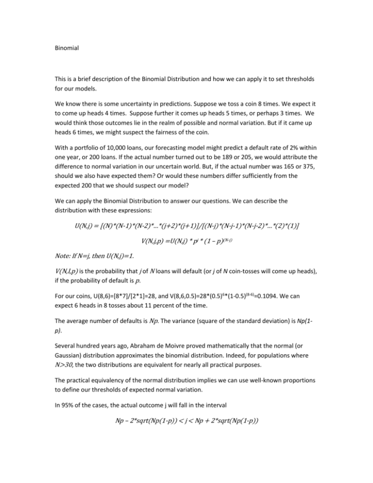
Binomial
This is a brief description of the Binomial Distribution and how we can apply it to set thresholds
for our models.
We know there is some uncertainty in predictions. Suppose we toss a coin 8 times. We expect it
to come up heads 4 times. Suppose further it comes up heads 5 times, or perhaps 3 times. We
would think those outcomes lie in the realm of possible and normal variation. But if it came up
heads 6 times, we might suspect the fairness of the coin.
With a portfolio of 10,000 loans, our forecasting model might predict a default rate of 2% within
one year, or 200 loans. If the actual number turned out to be 189 or 205, we would attribute the
difference to normal variation in our uncertain world. But, if the actual number was 165 or 375,
should we also have expected them? Or would these numbers differ sufficiently from the
expected 200 that we should suspect our model?
We can apply the Binomial Distribution to answer our questions. We can describe the
distribution with these expressions:
U(N,j) = [(N)*(N-1)*(N-2)*…*(j+2)*(j+1)]/[(N-j)*(N-j-1)*(N-j-2)*…*(2)*(1)]
V(N,j,p) =U(N,j) * pj * (1 – p)(N-j)
Note: If N=j, then U(N,j)=1.
V(N,I,p) is the probability that j of N loans will default (or j of N coin-tosses will come up heads),
if the probability of default is p.
For our coins, U(8,6)=[8*7]/[2*1]=28, and V(8,6,0.5)=28*(0.5)6*(1-0.5)(8-6)=0.1094. We can
expect 6 heads in 8 tosses about 11 percent of the time.
The average number of defaults is Np. The variance (square of the standard deviation) is Np(1p).
Several hundred years ago, Abraham de Moivre proved mathematically that the normal (or
Gaussian) distribution approximates the binomial distribution. Indeed, for populations where
N>30, the two distributions are equivalent for nearly all practical purposes.
The practical equivalency of the normal distribution implies we can use well-known proportions
to define our thresholds of expected normal variation.
In 95% of the cases, the actual outcome j will fall in the interval
Np – 2*sqrt(Np(1-p)) < j < Np + 2*sqrt(Np(1-p))
In 68% of the cases, the actual outcome j will fall in the interval
Np – 1*sqrt(Np(1-p)) < j < Np + 1*sqrt(Np(1-p))
For our N=10,000 loans with probability p=0.02 of default, we calculate
95% interval: 172 < j < 228
68% interval: 186 < j < 214
95% of cases will normally have 172 to 228 defaults.
68% of cases will normally have 186 to 214 defaults.
But 375 defaults won’t likely occur in 95 of 100 cases. If we see 375 actual defaults, then we
should suspect the model.
For our model performance thresholds, we can use the 95% and 68% intervals.
Thresholds
Actual < (Np - 2*sqrt(Np(1-p)))
or (Np + 2*sqrt(Np(1-p))) < Actual
(Np - 2*sqrt(Np(1-p))) <= Actual <= (Np - 1*sqrt(Np(1-p)))
or (Np + 1*sqrt(Np(1-p))) <= Actual <= (Np + 2*sqrt(Np(1-p)))
(Np - 1*sqrt(Np(1-p))) < Actual < (Np + 1*sqrt(Np(1-p)))
For more information, please see:
Charles Grinstead, J. Laurie Snell, Introduction to Probability, Second Revised Edition (American
Mathematical Society, 2003, retrieved 2011-12-16 from
http://www.dartmouth.edu/~chance/teaching_aids/books_articles/probability_book/amsbook.
mac.pdf); approximating Binomial Distribution with Normal Distribution: p. 329; Abraham de
Moivre: p. 337.
Richard Williams, The Binomial Distribution (University of Notre Dame, 2004, retrieved 2011-1216 from http://www.nd.edu/~rwilliam/stats1/x13.pdf), p. 11.