Introduction to SAS ® by Kaz Download from www.src.uchicago.edu/users/ueka
1
Introduction to SAS® Version 1.4 updated 9/29/2002
by Kazuaki Uekawa, Ph.D.
Visiting Scholar, The Department of Sociology, The
University of Chicago; Population Research Center at NORC; Address: 1155 E. 60th. St,
Room 340, Chicago, IL 60637
www.src.uchicago.edu/users/ueka
kuekawa@alumni.uchicago.edu
Copyright © 2002 By Kazuaki Uekawa All rights reserved.
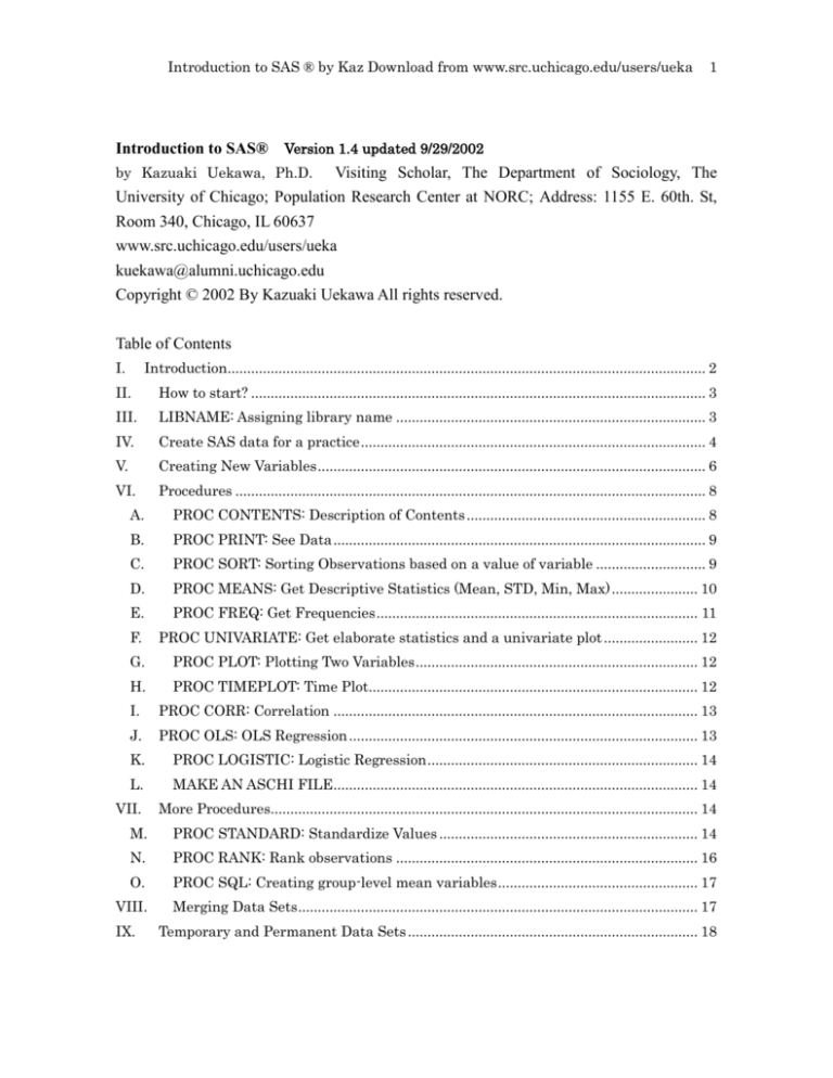
Table of Contents
I.
Introduction.......................................................................................................................... 2
II.
How to start? .................................................................................................................... 3
III.
LIBNAME: Assigning library name ............................................................................... 3
IV.
Create SAS data for a practice ........................................................................................ 4
V.
Creating New Variables ................................................................................................... 6
VI.
Procedures ........................................................................................................................ 8
A.
PROC CONTENTS: Description of Contents ............................................................. 8
B.
PROC PRINT: See Data ............................................................................................... 9
C.
PROC SORT: Sorting Observations based on a value of variable ............................ 9
D.
PROC MEANS: Get Descriptive Statistics (Mean, STD, Min, Max) ...................... 10
E.
PROC FREQ: Get Frequencies .................................................................................. 11
F.
PROC UNIVARIATE: Get elaborate statistics and a univariate plot ........................ 12
G.
PROC PLOT: Plotting Two Variables ........................................................................ 12
H.
PROC TIMEPLOT: Time Plot.................................................................................... 12
I.
PROC CORR: Correlation ............................................................................................. 13
J.
PROC OLS: OLS Regression ......................................................................................... 13
K.
PROC LOGISTIC: Logistic Regression ..................................................................... 14
L.
MAKE AN ASCHI FILE............................................................................................. 14
VII.
More Procedures............................................................................................................. 14
M.
PROC STANDARD: Standardize Values .................................................................. 14
N.
PROC RANK: Rank observations ............................................................................. 16
O.
PROC SQL: Creating group-level mean variables ................................................... 17
VIII.
Merging Data Sets ...................................................................................................... 17
IX.
Temporary and Permanent Data Sets .......................................................................... 18
Introduction to SAS ® by Kaz Download from www.src.uchicago.edu/users/ueka
2
I. Introduction
I recommend SAS® over other statistical packages because:
a) ODS (Output Delivery System) allows users to save statistical results as data. A
user can create tables off the result data set in one single program (as opposed to
printing out the results on paper and use excel to finish tables.) The table can be as
sophisticated as
http://www.src.uchicago.edu/users/ueka/SAS/proc_mixed_example1output.txt and
this can be further saved in an excel format using PROC EXPORT.
b) Rich arrays of macro functions
c) Email support service with quick response.
support@sas.com
d) Users come from many fields, including social and natural sciences, as well as
business. Thus, SAS ® programming skill can be an asset in the job market.
I discuss both ODS and MACRO in Introduction SAS 2, the document of which is
available from the same website.
Idiosyncrasy of this document
I am writing this document on my Japanese PC and backslash is not available.
I use
¥ instead.
U. of Chicago People can access SAS on-line on the web!
SAS On-line for version 8
http://gsbapp2.uchicago.edu/sas/sashtml/main.htm
Note on SAS email support:
When you email SAS support with a question, you need to identify yourself as a legitimate
SAS customer. Look at the head of a log file and copy and paste the information at the
beginning of your email text.
NOTE: Copyright (c) 1999-2001 by SAS Institute Inc., Cary, NC, USA.
NOTE: SAS (r) Proprietary Software Release 8.2 (TS2M0)
Licensed to UNIVERSITY OF XXXXX, Site XXXXX.
NOTE: This session is executing on the WIN_ME
platform.
Introduction to SAS ® by Kaz Download from www.src.uchicago.edu/users/ueka
3
II. How to start?
1. Start SAS. You can find the short cut going from START PROGRAMThe SAS
System.
2. Type in syntax in EDITOR window. Syntax is something you learn in this document.
3. Click on the runner icon to run the program. Alternatively, you can highlight the part of
syntax that you want to run and then click the runner to run the program selectively. (The
downside of using UNIX instead of WINDOWS is that UNIX cannot let you do this selective
run.)
LOG file contains messages. Watch for the words error and warning.
OUTPUT file contains output.
If you ever mistype syntax and want to redo, do control-z. This is the same
command that can be used with Microsoft Office products.
To cancel the run while it is happening, click on the stop icon (which looks
like “!”) right next to the runner icon.
III. LIBNAME: Assigning library name
Assigning library name
Using path names as directory names is too tedious (e.g., C: ¥temp¥abc¥old), so we want to
give nicknames to them at the beginning of a program.
libname here “C:¥TEMP”;
libname there “C:¥”;
So from now on,
here.abc means the data set named “abc” placed in the directory nicknamed “here.”
there.xyz means the data set named “xyz” placed in the directory nicknamed “there.”
Introduction to SAS ® by Kaz Download from www.src.uchicago.edu/users/ueka
4
IV. Create SAS data for a practice
Description of Practice Data
The data comes from TIMSS (Third International Mathematics and Science Study) in
which some 40 nations’ three population groups (3&4th graders, 7&8th graders, and high
school seniors) participated. I aggregated data at the national level. The variables are:
acro: acronym for participant nations.
nation: name of the country
name: complete name of the country
mat8: 8thgraders’ average math test score
mat7: 7thgraders’ average math test score
GNP14: GNP per capita
prop: proportion of 8th graders in schooling
NATEXA: Administers national-level exam
NATSYLB: Sylbus is decided at the national level
NATTEXT: text is chosen at the national level.
libname here “C:¥TEMP”;
libname there “C:¥”;
data kaz;
input
acro $ NATION $ 6-14
NAME
$
15-33
MAT7
MAT8
GNP14 PROP NATEXAM NATSYLB
NATTEXT block $;
cards;
aus
Australi Australia
498 529.63 -0.15526
84
0
1
0
ocea
aut
Austria
509 539.43 -0.29163
100
0
0
1
weuro
bfl
Belgi_FL Belgium (Fl)
558 565.18 -0.25157
100
1
1
0
weuro
bfr
Belgi_FR Belgium (Fr)
507 526.26 -0.25157
100
0
1
0
weuro
can
Canada
494 527.24
0.07184
88
0
0
0
namer
col
Colombia Colombia
369 384.76 -0.23699
62
0
1
0
samer
cyp
Cyprus
Cyprus
446 473.59 -0.41906
95
0
1
1
seuro
csk
Czech
Czech Republic
523 563.75 -0.34840
86
0
1
0
eeuro
dnk
Denmark
Denmark
465 502.29 -0.34057
100
1
0
0
weuro
Austria
Canada
Introduction to SAS ® by Kaz Download from www.src.uchicago.edu/users/ueka
fra
France
France
492 537.83
0.55791
100
0
1
0
weuro
deu
Germany
Germany
484 509.16
0.91992
100
0
0
0
weuro
grc
Greece
Greece
440 483.90 -0.32620
99
0
1
1
seuro
hkg
HongKong Hong Kong
564 588.02 -0.31638
98
1
1
1
seasia
hun
Hungary
Hungary
502 537.26 -0.37602
81
0
0
0
eeuro
isl
Iceland
Iceland
459 486.78 -0.42606
100
0
0
0
neuro
irn
Iran
Iran, Islamic Rep.
401 428.33 -0.17095
66
0
1
1
meast
irl
Ireland
Ireland
500 527.40 -0.38919
100
1
1
0
weuro
isr
Israel
Israel
. 521.59 -0.35464
87
0
1
0
meast
jpn
Japan
Japan
571 604.77
1.85543
96
0
1
0
seasia
kor
Korea
Korea
577 607.38 -0.01168
93
0
1
1
seasia
kwt
Kuwait
Kuwait
. 392.18 -0.40359
60
0
1
1
meast
lva
Latvia
Latvia (LSS)
462 493.36 -0.42319
87
0
0
0
eeuro
ltu
Lithuani Lithuania
428 477.23 -0.41785
78
1
1
1
eeuro
nld
Netherla Netherlands
516 540.99 -0.18184
93
1
0
0
weuro
nzl
NewZeala New Zealand
472 507.80 -0.38319
100
1
1
0
ocea
nor
Norway
461 503.29 -0.35450
100
0
1
1
neuro
prt
Portugal Portugal
423 454.45 -0.32588
81
0
1
0
weuro
rom
Romania
454 481.55 -0.35396
82
1
1
1
eeuro
rus
RussianF Russian Federation
501 535.47
0.12827
88
1
0
0
eeuro
sco
Scotland Scotland
463 498.46
0.48017
100
0
0
0
weuro
sgp
Singapor Singapore
601 643.30 -0.37279
84
1
1
1
seasia
slv
SlovakRe Slovak Republic
508 547.11 -0.40217
89
0
1
0
eeuro
svn
Slovenia Slovenia
498 540.80 -0.41310
85
0
1
1
eeuro
esp
Spain
Spain
448 487.35
0.03461
100
0
1
1
weuro
swe
Sweden
Sweden
477 518.64 -0.30049
99
0
1
0
neuro
che
Switzerl Switzerland
506 545.44 -0.27916
91
0
0
0
weuro
tha
Thailand Thailand
495 522.37 -0.14533
37
0
1
1
seasia
usa
USA
476 499.76
97
0
0
0
namer
Norway
Romania
United States
;
run;
/*this prints out the data*/
proc print;
run;
5.37506
5
Introduction to SAS ® by Kaz Download from www.src.uchicago.edu/users/ueka
6
Advanced Topic:
Alternatively you can save above data (just data part) as a simple text and save it at your
C-drive’s temp directory as kaz.txt. (In case you only have this document as a hard copy,
visit www.src.uchicago.edu/users/ueka for a digital version of this document, so you can
copy and paste.) Then use the program below to read in the file.
/*these two lines are not crucial in this example, but let’s just put these at the beginning of
your program*/
libname here “C:¥TEMP”;
libname there “C:¥”;
data kaz;
infile “C:¥TEMP¥kaz.txt” missover;
input
acro $ NATION $ 6-14
NAME $
15-33
MAT7
GNP14
PROP NATEXAM NATSYLB NATTEXT block $;
MAT8
run;
I think missover means that when there is no value in the spot where there is supposed to be
a value, just treat it as a missing value, but I forgot exactly. It is safe to use it.
$ means whatever comes before it is a character variable as opposed to numeric.
V. Creating New Variables
Data kaz2;
set kaz;
/*ADDITION*/
var1=mat7+mat8;
Introduction to SAS ® by Kaz Download from www.src.uchicago.edu/users/ueka
7
/*OR*/
var2=sum(of mat7 mat8);
/*SUBSTRACTION*/
var3=mat8-mat7;
/*MULTIPLICATION*/
var4=mat7*mat8;
/*DIVISION*/
var5=mat7/mat8;
/*LOG: a value to enter must be
positive*/
var10=log(mat7);
/*Absolute values: this takes out negative
signs*/
var11=abs(gnp14);
run;
/*Use brackets effectively*/
var6=1/(mat7+mat8);
/*MEAN of several variables*/
var7=mean(of mat7 mat8);
/*MAX of several variables*/
var8=max(of mat7 mat8);
/*MIN of several variables*/
var9=min(of mat7 mat8);
/*TO SEE WHAT YOU DID, USE PROC
PRINT*/
proc print data=kaz2;
title “Lots of manipulations: See results”;
var mat7 mat8 var1 var2 var3 var4 var5
var6 var7 var8 var9 var10 var11;
run;
Advanced Topics:
How is Z=mean(of X1 X2 X3) different from Z=(X1+X2+X3)/2;?
How is Z=sum(of X1 X2 X3) different from Z=X1+X2+X3;?
Functions, such as mean(of …) or sum (of …), take statistics of non-missing values. They
do return values even when some of the variables in the brackets are missing. For
example, if X1 is missing:
X=mean (of X1 X2 X3); will return the average of X2 and X3.
In contrast,
X=(X1+X2+X3)/2 will return a missing value, namely, “.”
Read this after you study PROC REG later in the document.
When we compare several regression models (e.g., coefficients, R2, Goodness-of-fit, etc.),
we want to keep the number of observations same across different models. Because
Introduction to SAS ® by Kaz Download from www.src.uchicago.edu/users/ueka
8
predictors may have different patterns of missing values, this must be made to happen if
you want to. For example, mat7, which is 7th graders’ mathematics score include some
missing cases. Some nations only let their 8th graders participate in this international test.
Use NMISS function to create a new variable john.
data kaz2;set kaz;
john=nmiss(of GNP14 mat8 mat7);/*this returns the number of missing cases*/
run;
/*check how the data looks like now*/
proc print data=kaz2;
var name gnp14 mat8 mat7 john;
run;
/*Apply OLS regression with cases with perfect data (no missing cases). In this way,
model 1 and model 2 will have the same number of cases, or to be more precise, the same
data.*/
proc reg data=kaz2;
where john=0; /*Run only when john=0, namely, number of missing cases is 0*/
model mat8=mat7;
model mat8=mat7 gnp14;
run;
VI. Procedures
A. PROC CONTENTS: Description of Contents
PROC CONTENTS data=kaz;
run;
Advanced topic: the variables will be sorted by alphabetical order.
They can be also
shown by position in the data set (left to right) by addition “position”:
proc contents data=kaz position;
Introduction to SAS ® by Kaz Download from www.src.uchicago.edu/users/ueka
9
run;
I like this option because in this way you can find related variables close to each other.
B. PROC PRINT: See Data
PROC PRINT data=kaz;
VAR nation mat7 mat8 natexam; /*without this, all variables will be printed*/
run;
Advanced topic: You can selectively print observations.
/*print only when natexam=1*/
proc print data=kaz;where natexam=1;var nation mat7 mat8;run;
/*print by group units*/
proc sort data=kaz out=kaz2;by block;run;
proc print data=kaz;by block;var nation mat7 mat8;run;
/*print only up to a certain number of observations*/
proc print data=kaz2 (obs=5); /*shows only five observations*/
run;
If you want a nicer print-out, try proc report.
C. PROC SORT: Sorting Observations based on a value of variable
You would be using this procedure a lot, but be careful with large data set. This procedure
consumes lots of computation time.
PROC SORT data=kaz out=kaz2;
/*If you don’t want to create a new data set, just write “out=kaz”*/
by mat8;
run;
Advanced topics:
proc sort data=kaz out=kaz2 nodupkey;
by block;
run;
Introduction to SAS ® by Kaz Download from www.src.uchicago.edu/users/ueka 10
proc print data=kaz2;run;
This takes only the first observation of each block. Imagine that you have data where
there are individual level variable (e.g., 100 students) and group level variable (e.g., 10
schools).
Imagine you want to get school level information from this data.
Above
procedure would take just the first observation of each school and gets you ten lines of data
for 10 schools. Ignore individual-level variables, however.
You can use more than one variable in by line.
proc sort data=kaz out=kaz2;
by natexam block;
run;
/*How would the new data look like?*/
proc print data=kaz2;run;
D. PROC MEANS: Get Descriptive Statistics (Mean, STD, Min, Max)
PROC MEANS data=kaz;
VAR mat7 mat8;
run;
Advanced topic: Group means.
/*Report group means*/
proc sort data=kaz out=kaz2;by block;run;
proc means data=kaz2;
by block;
var mat7 mat8;
run;
You can also use “class” statement instead of “by” statement. Class statement is easier
Introduction to SAS ® by Kaz Download from www.src.uchicago.edu/users/ueka 11
because you don’t need to sort the data by the by-variable before it.
downside of it was.
I forgot what the
proc means data=kaz2; /*now, kaz2 does not have to be sorted by block*/
class block;
var mat7 mat8;
run;
/*Save group means*/
ods listing close; /*printing of results suppressed*/
proc means data=kaz2; /*make sure kaz2 is already sorted by group ID*/
by block;
var mat7 mat8;
ods output summary=john; /*Output Delivery System Used. See SAS manual 2*/
run;
ods listing on; /*printing of results resumed*/
proc print data=john;
run;
/*Get standard errors by adding STDERR*/
/*But it would only get standard error, so you must add other statistics you would like with
it. Specify mean, N, STD, MAX, and MIN*/
PROC MEANS data=kaz mean n std max min stderr;
VAR mat7 mat8;run;
run;
I recommend reading a chapter on PROC MEANS in SAS CD-online. It is a very
versatile procedure.
E. PROC FREQ: Get Frequencies
PROC FREQ data=kaz;
Tables natexam ;
Introduction to SAS ® by Kaz Download from www.src.uchicago.edu/users/ueka 12
Run;
Advanced topics:
Get cross tabulation:
PROC FREQ data=kaz;
tables natexam*block;
run;
F. PROC UNIVARIATE: Get elaborate statistics and a univariate plot
PROC UNIVARIATE PLOT DATA=KAZ;
var mat7 mat8 gnp14;
run;
Advanced topic:Get a whisker plot by sub groups, so you can compare group values. But
the output is text-based and pretty ugly.
proc sort data=kaz out=kaz2;
by block;
run;
PROC UNIVARIATE data=kaz2 plot;
by block;
var mat8;
run;
G. PROC PLOT: Plotting Two Variables
This is text-based graph. Use proc gplot for a nicer graphic.
PROC PLOT data=KAZ;
Plot mat7*mat8;
run;
H. PROC TIMEPLOT: Time Plot
proc timeplot data=KAZ;
plot mat8= '*';
id NAME;
run;
Advanced topics:
Introduction to SAS ® by Kaz Download from www.src.uchicago.edu/users/ueka 13
/*Sort first by the variable of your interest and see it*/
/*you will be seeing a ranking of nations*/
proc sort data=kaz out=kaz2;
by mat8;
run;
proc timeplot data=KAZ2;
plot mat8= '*';
id NAME;
run;
Add bells and whistles. Below, I am asking, “Does GNP has anything to do with test
score?
/*First sort by GNP*/
proc sort data=kaz out=kaz2;
by gnp14;
run;
proc timeplot data=KAZ2;
title “TIMSS countries sorted by GNP”;
plot mat7 mat8/overlay hiloc npp ;
id NAME block gnp14 prop;
run;
I. PROC CORR: Correlation
PROC CORR DATA=KAZ;
VAR mat7 mat8 gnp14;
Run;
J. PROC OLS: OLS Regression
PROC REG DATA=KAZ;
MODEL mat8=natexam gnp14;
Run;
Advanced Topic:
See www.src.uchicago.edu/users/ueka for the creation of OLS table using OLS. Also see
PROC IML instruction on the same page to learn how OLS estimates its coefficients.
Introduction to SAS ® by Kaz Download from www.src.uchicago.edu/users/ueka 14
K. PROC LOGISTIC: Logistic Regression
/*I don’t know if natexam can be considered a dependent variable, but for the sake of
demonstration*/
PROC logistic data=kaz descend;
Model natexam=gnp14;
run;
/*option descend makes sure that RROC LOGISTIC is modeling the probability that the
outcome=1. Without this option, it would model the probability that the outcome=0*/
L. MAKE AN ASCHI FILE
To use a stand-alone software program, you may have to create a simple aschi file. But I
rarely use this lately because many software read SAS data directly.
data timss;set kaz;
file "aschi_example.txt";
put (nation) (10.0) (mat7 mat8) (8.0);
run;
VII. More Procedures
M. PROC STANDARD: Standardize Values
Make Z-score with a mean of 0 and standard deviation of 1
proc standard data=kaz out=kaz2 mean=0 std=1;
var mat7 mat8;
run;
/*then see what you did*/
proc print data=kaz2;
run;
Advanced technique: Standardize within groups.
/*First sort by group ID*/
proc sort data=kaz out=kaz2;
Introduction to SAS ® by Kaz Download from www.src.uchicago.edu/users/ueka 15
by block;
run;
/*Use by statement*/
proc standard data=kaz2 out=kaz3 mean=0 std=1;
by block;
var mat7 mat8;
run;
Introduction to SAS ® by Kaz Download from www.src.uchicago.edu/users/ueka 16
N. PROC RANK: Rank observations
proc rank data=kaz out=kaz2 group=3;
/*Creates 3 groups. The new values will be 0, 1, and 2. */
var mat7 mat8;
RANKS Rmat7 Rmat8;
/*give names to the new variables*/
Run;
/*see what happened*/
proc print data=kaz2;
var mat7 Rmat7 mat8 Rmat8;
RUN;
Research Tip:
Why do we use rank?
a. We can split the sample based on the rank. e.g., high SES student sample versus low
SES student sample.
b. We can create dummy variables quickly by specifying group=2. e.g., high SES student
will receive 1; else 0. This grouping occurs at the median point of a variable, which may
or may not be always the best strategy. Alternative way is to assign 1 and 0 based on
some meaningful threshold. For example, I have temperature data, I may use a medium
point to split the data if it makes sense, but maybe I use 0 degree (Freezing point) as a
meaningful point to split the data instead.
Introduction to SAS ® by Kaz Download from www.src.uchicago.edu/users/ueka 17
O. PROC SQL: Creating group-level mean variables
One could use proc means to derive group-level means. I don’t recommend this since it
involves extra steps of merging the mean data back to the main data set. Extra steps
always create rooms for errors. PROC SQL does it at once.
proc sql;
create table kaz2 as
select *,
mean(mat7) as mean_mat7,
mean(mat8) as mean_mat8,
mean(gnp14) as mean_gnp
from kaz
group by block;
run; /*proc sql does not really require run statement, but for the sake of consistency*/
proc print data=kaz2;
run;
VIII. Merging Data Sets
libname here “C:¥”;
/*Create two data sets A and B.*/
data A;
set kaz; /*I am assuming that you already have this data set “kaz” by running the program
on page 4 and 5 of this document. */
keep nation mat7;
run;
Introduction to SAS ® by Kaz Download from www.src.uchicago.edu/users/ueka 18
data B;
set kaz;
keep nation mat8;
run;
/*MERGE DATA SETS*/
/*First sort them by a common ID*/
/*Here they are already sorted, so the following two lines are not really necessary*/
proc sort data=A;by nation;run;
proc sort data=B;by nation;run;
data NEW;
merge A B;
by nation;
run;
/*Confirm*/
proc print data=NEW;
run;
IX. Temporary and Permanent Data Sets
There are temporary and permanent SAS data sets. When you turn off SAS, the
temporary data will be erased. Throughout the exercise, you have seen “kaz” and “kaz2.”
They are temporary data sets.
To actually see these data, go to the Explorer (leftish side of the SAS window),
then to Libraries, and find folders in there. The default directory is called Work. (You
will also find folders that you nicknamed.) Click them to open and find data in them.
If you want to make them permanent, so they don’t disappear when you turn off
SAS, add the directory nickname in front of the new data set.
For example:
Data here.abc;set kaz;
keep nation growth;
growth=mat8-mat7;
run;
You are bringing in a temporary data set “kaz” and are creating a new permanent data
called abc in the directory “C:¥TEMP” (nicknamed “here” by a library statement) You are
Introduction to SAS ® by Kaz Download from www.src.uchicago.edu/users/ueka 19
creating a variable called “growth” and it now is in here.abc. Only nation and growth are
kept in the new data set.
You can also do the opposite: bring in a permanent data set this time and create a temporary
data.
Data xyz; set here.abc;
growth=mat8-mat7;
drop mat8 mat7;
run;
You are bringing a permanent data set called “abc” placed in C:¥TEMP and create a new
data abc in SAS’s defalt directory. You created a variable called “growth” and it now is in
abc. Mat8 and mat7 are dropped from the new data set.
(Of course, reading in a permanent data and creating a permanent data is possible by “data
here.xyz; set here.xyz;)
Research Tip:
I recommend that you make permanent data as infrequently as possible. Just save your
syntax program and create fresh temporary data each time you start and save disc space..
In this way, you can just save your small syntax program. Also research is a lot easier if
you have only a few programs and data sets.
http://www.src.uchicago.edu/users/ueka/SAS/Dataextractor8.3.txt
Every time I need to work on this study, I can just run this one single program to reproduce
data. I don’t have to remember the name convention and location of the data sets that I
have to deal with.
For this particular study, I only need to deal with this file above and one more file
that actually does the analyses.
http://www.src.uchicago.edu/users/ueka/SAS/MakeFinalTables7.2.txt
If I need to make changes to my analyses, I know I just have to look into these two
files. This would be impossible if I had too many files and data sets flying all over the
places even in one directory.
Introduction to SAS ® by Kaz Download from www.src.uchicago.edu/users/ueka 20
HOWEVER, if your data is huge (e.g., census data), then you may be better off
saving permanent data, so it is quicker.
END of Document
