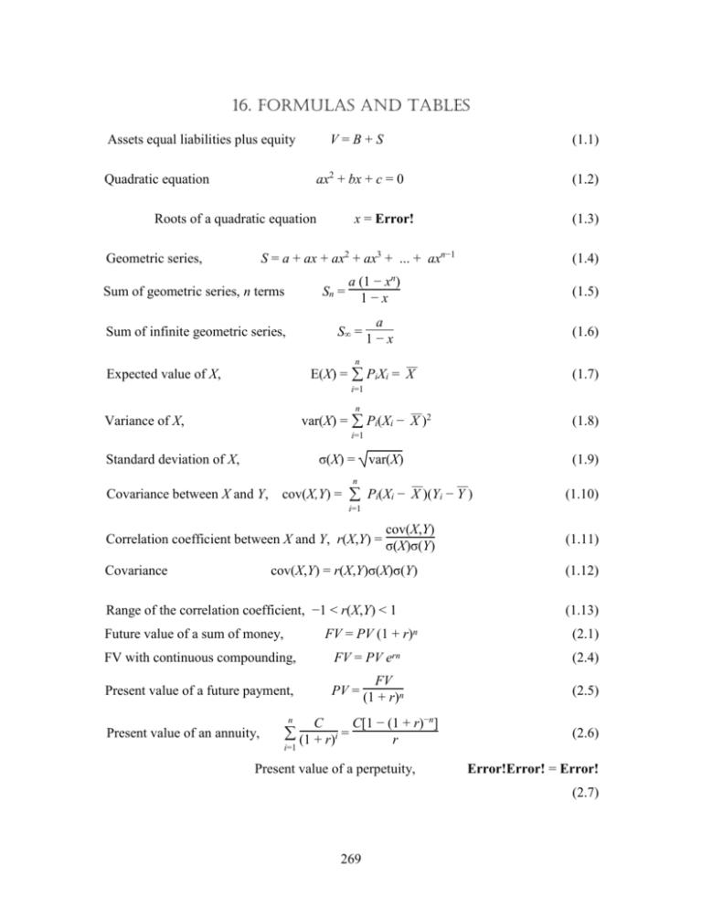
16. FORMULAS AND TABLES
Assets equal liabilities plus equity
Quadratic equation
V=B+S
(1.1)
ax2 + bx + c = 0
(1.2)
Roots of a quadratic equation
x = Error!
(1.3)
S = a + ax + ax2 + ax3 + ... + axn−1
Geometric series,
Sum of geometric series, n terms
Sn =
(1.4)
a (1 − xn)
1−x
(1.5)
a
S∞ = 1 − x
Sum of infinite geometric series,
(1.6)
n
—
E(X) =  PiXi = X
Expected value of X,
(1.7)
i=1
n
—
var(X) =  Pi(Xi − X )2
Variance of X,
(1.8)
i=1
σ(X) = var(X)
Standard deviation of X,
Covariance between X and Y,
(1.9)
n
—
—
cov(X,Y) =  Pi(Xi − X )(Yi − Y )
(1.10)
i=1
cov(X,Y)
Correlation coefficient between X and Y, r(X,Y) = σ(X)σ(Y)
(1.11)
Covariance
(1.12)
cov(X,Y) = r(X,Y)σ(X)σ(Y)
Range of the correlation coefficient, −1 < r(X,Y) < 1
FV = PV (1 + r)n
Future value of a sum of money,
(1.13)
(2.1)
FV with continuous compounding,
FV = PV ern
(2.4)
Present value of a future payment,
FV
PV = (1 + r)n
(2.5)
n
Present value of an annuity,
C
 (1 + r)i =
i=1
C[1 − (1 + r)−n]
r
Present value of a perpetuity,
(2.6)
Error!Error! = Error!
(2.7)
269
Analytical Techniques
16. Formulas and Tables
_____________________________________________________________________________
n
1
C
PV of n cash flows, starting after k periods, PV = (1 + r)k–1  (1 + r)i
i=1
(2.8)
C(1 + r)[(1 + r)n – 1]
r
(2.9)
Future value of n cash flows, starting now, FV =
n
P
L =  (1 + r)i
Loan amortization,
(2.10)
i=1
n
P
B
Loan amortization with balloon payment B, L =  (1 + r)i + (1 + r)n
(2.11)
n
w 

n
Future value, including withdrawals, FV = A − 
i(1 + r)
(1
+
r)


i=1
(2.12)
i=1
 w 
lnw – Ar


n = ln(1 + r)
Time to exhaust savings,
n
C
F
Present value of a coupon bond, B =  (1 + r)i + (1 + r)n
(2.13)
(3.1)
i=1
C
B= r
Present value of a perpetual bond,
Present value of a zero-coupon bond,
B=
Current yield of a bond,
F
(1 + r)n
y = cF/B
Gordon's growth model,
Net present value,
(3.3)
(3.4)
cF + (F − B)/n
(F + B)/2
(3.5)
D1
P0 = R − g
(3.6)
n
C
NPV = − I0 +  (1 + r)i
(4.1)
Y≈
Yield-to-maturity of a bond,
(3.2)
i=1
n
Internal rate of return,
C
(1
+
IRR)i
i=1
NPV = 0 =  I0 + 
After-tax cash flow,
With maintenance cost M,
C = E(1 − t) + tD
C = (1t)(E  M) + tD
(4.2)
(4.3)
(4.4)
Book value of an asset,
B = I0 – nD
(4.5)
Tax due on the sale of an asset,
T = t(S  B)
(4.6)
After-tax value of resale price,
W = S(1 – t) + tB
(4.7)
270
Analytical Techniques
16. Formulas and Tables
_____________________________________________________________________________
For a two-security portfolio,
w1 + w2 = 1
(6.6)
E(Rp) = w1 E(R1) + w2 E(R2)
(6.7)
σ(Rp) = w12 σ12 + w22 σ22 + 2w1w2 σ1σ2r12
(6.8)
cov(i,j) = σiσjrij
Covariance between i and j,
(6.5)
n
 wi = 1
For an n security portfolio,
(6.12)
i=1
n
E(Rp) =  wi E(Ri)
Expected return of portfolio,
(6.13)
i=1
[
n
]
n
σ(Rp) =   wiwjcov(i,j)
Its standard deviation,
i=1 j=1
1/2
(6.5)
n
E(Rp) =  E(Ri)
For dollar amounts,
(6.18)
i=1
[
n
n
]
σ(Rp) =   cov(i,j)
Return on a stock,
Return on the market,
Definition of β,
i=1 j=1
1/2
(6.19)
Rj =
P1 − P0 + D1
P0
(7.1)
Rm =
M1 − M0
M0 + d1
(7.2)
cov(Rj,Rm) rjmσmσj rjmσj
βj = var(R ) = σ 2 = σ
m
m
m
Calculation of β,
β=
Calculation of α,
(7.3)
n(xy) − (x)(y)
nx2 − (x)2
α=
(7.4)
y − βx
(7.5)
n
n
Beta of a portfolio,
βp = w1β1 + w2β2 + w3β3 + ... =  wiβi
(7.6)
i=1
Capital Asset Pricing Model,
E(Ri) = r + βi [E(Rm) − r]
(7.7)
Black-Scholes model,
C = S N(d1) − X e−rT N(d2)
(8.3)
where
d1 =
ln(S/X) + (r + σ2/2)T
σ T
271
(8.4)
Analytical Techniques
16. Formulas and Tables
_____________________________________________________________________________
and
d2 =
ln(S/X) + (r − σ2/2)T
= d1 − σ T
σ T
P + S = C + X e−rT
Put-Call Parity Theorem,
(8.7)
Value of a European put, P = S [N(d1) – 1] − X e−rT [N(d2) −1]
(8.11)
V=B+S
(9.4)
B
S
WACC = (1 − t) kd V + ke V
(9.5)
EAT
EPS = N
(10.1)
EAT = (EBIT − I)(1 − t)
(10.2)
(EBIT − I) (1 − t) − SF − PD
N
(10.3)
(EBIT − I − r F) (1 − t) − SF − PD
N
(10.4)
Total value of a firm,
Earnings per share,
Earnings after taxes,
Earnings per share,
Bond financing,
Stock financing,
EPS =
EPS(bonds) =
EPS(stock) =
Critical EBIT,
(EBIT − I) (1 − t) − SF − PD
N + F/P
E* = I + r(NP + F) +
For SF = PD = 0,
(8.8)
∂C
h = ∂S = N(d1)
Hedge ratio,
WACC,
(8.5)
SF + PD
1−t
(10.5)
(10.6)
E* = I + r (N P + F)
(10.7)
Tax shield = tB
(10.8)
Value of a leveraged firm,
VL = VU + tB − b
(10.9)
Change in the value of a firm
ΔVL = tΔB − Δb
[
(10.10)
]
B
βL = βU 1 + (1 − t) S
Leveraged beta,
12(R − M)(1 − t) + tD Hn − (Hn − H + nD)t
+
(1 + r)i
(1 + r)n
i=1
(11.3)
n
House, H
NPV = − H + 
272
(14.2)
Analytical Techniques
16. Formulas and Tables
_____________________________________________________________________________
16.1
How to Use the Probability Tables
In some finance problems, you need to estimate the probability of something happening.
For example, a typical question is to find the probability that a given machine may run
for more than 5 years. If we assume that the life of the machine is normally distributed,
and we know the two parameters that describe the distribution, namely the expected value
μ and the standard deviation, σ, then we can answer the question. Further, you need to
learn the use of the probability tables or the NORMDIST function in Excel. The tables
are a little easier to use, although Excel does the calculations automatically.
Suppose you have a portfolio whose expected return is 11%, with normal distribution and
a standard deviation of 7%. You want to find the probability that, by chance, it will
provide a return of 15% or higher. By reading the problem, you know that it is unlikely to
happen. You expect to have a return of 11%, but you require a return of 15%. The result
should be less than 50%.
Start by calculating the parameter z = |μ − x|/σ. It comes out as z = |.11 − .15|/.07 = 4/7 =
.5714285716. Let us truncate it to four figures because that is the accuracy of the tables.
Thus z = .5714.
Next, draw a bell-shaped probability distribution curve. Put z = 0 at the center and mark
off points at −3, −2, −1, 0, 1, 2, and 3. These points are σ, 2σ, and 3σ from the center. The
required return is .15, which is equivalent to z = .5714. It is about ½σ away from the
center. Since we need the probability of return to be higher than .15, we need the area to
the right of z = .5714, which is under the tail of the curve.
The tables are set up to provide the area from the center to the point z. In our case, z =
.5714. To read the tables, first find the area for the first two digits, .57 and then add to it,
14% of the difference between the areas corresponding to .58 and .57. The number 14%
comes from the last two digits of z = .5714. This gives the required area for .5714.
Whatever area we get, we have to subtract it out .5 to find the area under the tail of the
curve. Put it all together as follows:
P(R > .15) = .5 – [.2157 + .14(.2190 − .2157)] = .2838 = 28.38% ♥
273
Analytical Techniques
16. Formulas and Tables
_____________________________________________________________________________
The portfolio with expected return 11%, and standard deviation 7%, has 28.38%
probability that it may actually attain a return of 15% or higher. This is a reasonable
answer.
You will need the table to find the values of N(d1) and N(d2) for use in the Black-Scholes
model. In this case N(d1) and N(d2) represent the total area under the normal probability
curve, measured from −∞ up to the point d1 or d2. Suppose d1 = .5462, which is positive.
You can place it to the right of zero, or the midpoint of the curve. In this case the area
N(d1) will be somewhat more than .5, as shown in the following diagram.
By the use of the tables, we get
N(d1) = .5 + .2054 + .62(.2088 − .2054) = .7075
If d2 is negative, say, −.4142, then it will lie on the left side of the center of the curve.
The shaded area will be less than .5, as seen the next diagram.
The result in this case will be
N(d2) = .5 – [.1591 + .42(.1628 − .1591)] = .3393 ♥
274
Analytical Techniques
16. Formulas and Tables
_____________________________________________________________________________
Area under the normal probability curve, from the center to a point z, where z =
x−μ
σ
z
0.01
0.02
0.03
0.04
0.05
Area
.0040
.0080
.0120
.0160
.0199
z
0.51
0.52
0.53
0.54
0.55
Area
.1950
.1985
.2019
.2054
.2088
z
1.01
1.02
1.03
1.04
1.05
Area
.3438
.3461
.3485
.3508
.3531
z
1.51
1.52
1.53
1.54
1.55
Area
.4345
.4357
.4370
.4382
.4394
z
2.01
2.02
2.03
2.04
2.05
Area
.4778
.4783
.4788
.4793
.4798
z
2.51
2.52
2.53
2.54
2.55
Area
.4940
.4941
.4943
.4945
.4946
0.06
0.07
0.08
0.09
0.10
.0239
.0279
.0319
.0359
.0398
0.56
0.57
0.58
0.59
0.60
.2123
.2157
.2190
.2224
.2257
1.06
1.07
1.08
1.09
1.10
.3554
.3577
.3599
.3621
.3643
1.56
1.57
1.58
1.59
1.60
.4406
.4418
.4429
.4441
.4452
2.06
2.07
2.08
2.09
2.10
.4803
.4808
.4812
.4817
.4821
2.56
2.57
2.58
2.59
2.60
.4948
.4949
.4951
.4952
.4953
0.11
0.12
0.13
0.14
0.15
.0438
.0478
.0517
.0557
.0596
0.61
0.62
0.63
0.64
0.65
.2291
.2324
.2357
.2389
.2422
1.11
1.12
1.13
1.14
1.15
.3665
.3686
.3708
.3729
.3749
1.61
1.62
1.63
1.64
1.65
.4463
.4474
.4484
.4495
.4505
2.11
2.12
2.13
2.14
2.15
.4826
.4830
.4834
.4838
.4842
2.61
2.62
2.63
2.64
2.65
.4955
.4956
.4957
.4959
.4960
0.16
0.17
0.18
0.19
0.20
.0636
.0675
.0714
.0753
.0793
0.66
0.67
0.68
0.69
0.70
.2454
.2486
.2517
.2549
.2580
1.16
1.17
1.18
1.19
1.20
.3770
.3790
.3810
.3830
.3849
1.66
1.67
1.68
1.69
1.70
.4515
.4525
.4535
.4545
.4554
2.16
2.17
2.18
2.19
2.20
.4846
.4850
.4854
.4857
.4861
2.66
2.67
2.68
2.69
2.70
.4961
.4962
.4963
.4964
.4965
0.21
0.22
0.23
0.24
0.25
.0832
.0871
.0910
.0948
.0987
0.71
0.72
0.73
0.74
0.75
.2611
.2642
.2673
.2704
.2734
1.21
1.22
1.23
1.24
1.25
.3869
.3888
.3907
.3925
.3944
1.71
1.72
1.73
1.74
1.75
.4564
.4573
.4582
.4591
.4599
2.21
2.22
2.23
2.24
2.25
.4864
.4868
.4871
.4875
.4878
2.71
2.72
2.73
2.74
2.75
.4966
.4967
.4968
.4969
.4970
0.26
0.27
0.28
0.29
0.30
.1026
.1064
.1103
.1141
.1179
0.76
0.77
0.78
0.79
0.80
.2764
.2794
.2823
.2852
.2881
1.26
1.27
1.28
1.29
1.30
.3962
.3980
.3997
.4015
.4032
1.76
1.77
1.78
1.79
1.80
.4608
.4616
.4625
.4633
.4641
2.26
2.27
2.28
2.29
2.30
.4881
.4884
.4887
.4890
.4893
2.76
2.77
2.78
2.79
2.80
.4971
.4972
.4973
.4974
.4974
0.31
0.32
0.33
0.34
0.35
.1217
.1255
.1293
.1331
.1368
0.81
0.82
0.83
0.84
0.85
.2910
.2939
.2967
.2995
.3023
1.31
1.32
1.33
1.34
1.35
.4049
.4066
.4082
.4099
.4115
1.81
1.82
1.83
1.84
1.85
.4649
.4656
.4664
.4671
.4678
2.31
2.32
2.33
2.34
2.35
.4896
.4898
.4901
.4904
.4906
2.81
2.82
2.83
2.84
2.85
.4975
.4976
.4977
.4977
.4978
0.36
0.37
0.38
0.39
0.40
.1406
.1443
.1480
.1517
.1554
0.86
0.87
0.88
0.89
0.90
.3051
.3078
.3106
.3133
.3159
1.36
1.37
1.38
1.39
1.40
.4131
.4147
.4162
.4177
.4192
1.86
1.87
1.88
1.89
1.90
.4686
.4693
.4699
.4706
.4713
2.36
2.37
2.38
2.39
2.40
.4909
.4911
.4913
.4916
.4918
2.86
2.87
2.88
2.89
2.90
.4979
.4979
.4980
.4981
.4981
0.41
0.42
0.43
0.44
0.45
.1591
.1628
.1664
.1700
.1736
0.91
0.92
0.93
0.94
0.95
.3186
.3212
.3238
.3264
.3289
1.41
1.42
1.43
1.44
1.45
.4207
.4222
.4236
.4251
.4265
1.91
1.92
1.93
1.94
1.95
.4719
.4726
.4732
.4738
.4744
2.41
2.42
2.43
2.44
2.45
.4920
.4922
.4925
.4927
.4929
2.91
2.92
2.93
2.94
2.95
.4982
.4982
.4983
.4984
.4984
0.46
0.47
0.48
0.49
0.50
.1772
.1808
.1844
.1879
.1915
0.96
0.97
0.98
0.99
1.00
.3315
.3340
.3365
.3389
.3413
1.46
1.47
1.48
1.49
1.50
.4279
.4292
.4306
.4319
.4332
1.96
1.97
1.98
1.99
2.00
.4750
.4756
.4761
.4767
.4772
2.46
2.47
2.48
2.49
2.50
.4931
.4932
.4934
.4936
.4938
2.96
2.97
2.98
2.99
3.00
.4985
.4985
.4986
.4986
.4987
275