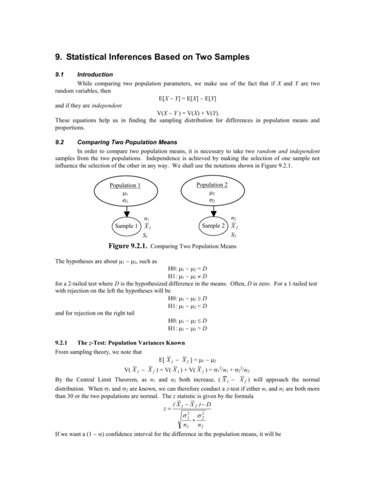
9. Statistical Inferences Based on Two Samples
9.1
Introduction
While comparing two population parameters, we make use of the fact that if X and Y are two
random variables, then
E[X Y] = E[X]  E[Y]
and if they are independent
V(X Y ) = V(X) + V(Y).
These equations help us in finding the sampling distribution for differences in population means and
proportions.
9.2
Comparing Two Population Means
In order to compare two population means, it is necessary to take two random and independent
samples from the two populations. Independence is achieved by making the selection of one sample not
influence the selection of the other in any way. We shall use the notations shown in Figure 9.2.1.
Population 2
2
2
Population 1
1
1
Sample 1
n1
X1
S1
Sample 2
n2
X2
S2
Figure 9.2.1. Comparing Two Population Means
The hypotheses are about 1 2, such as
H0: 1 2 = D
H1: 1 2  D
for a 2-tailed test where D is the hypothesized difference in the means. Often, D is zero. For a 1-tailed test
with rejection on the left the hypotheses will be
H0: 1 2  D
H1: 1 2 < D
and for rejection on the right tail
H0: 1 2  D
H1: 1 2 > D
9.2.1
The z-Test: Population Variances Known
From sampling theory, we note that
E[ X 1  X 2 ] = 1  2
V( X 1  X 2 ) = V( X 1 ) + V( X 2 ) = 12/n1 + 22/n2.
By the Central Limit Theorem, as n1 and n2 both increase, ( X 1  X 2 ) will approach the normal
distribution. When 1 and 2 are known, we can therefore conduct a z-test if either n1 and n2 are both more
than 30 or the two populations are normal. The z statistic is given by the formula
( X1  X2 ) D
z
 12
n1

 22
n2
If we want a (1 ) confidence interval for the difference in the population means, it will be
52
( x 1  x 2 )  z / 2
 12
n1

 22
n2
.
The template is shown in Figure 9.2.2. After entering the input data in the shaded cells, the p-values of
hypothesis tests and the confidence intervals appear at the designated places.
Note: The user may have to calculate the sample means and then input them into cells B6 and E6.
If the raw data from the samples are entered in another area of the sheet and are named “Sample1” and
“Sample2”, then the formula =AVERAGE(Sample1) may be entered in cell B6, and the formula
=AVERAGE(Sample2) in cell E6. One may also use the COUNT function to calculate the sample sizes.
For instance, the formula =COUNT(Sample1) would return n1. While entering population variance, one
should make sure that it is the variance (and not the standard deviation).
Figure 9.2.2. z-Test for Difference in Population Means
[Workbook: Testing Differences.xls; Sheet: z-Test]
9.2.2
The t-Test: Population Variances Unknown
The z-test is possible only when the population variances are known, but very often they are
unknown. If they are unknown, a t-test is possible. Here there are two cases, one where the population
variances are assumed to be equal and the other where they are assumed to be unequal. The assumption of
equal variances is justified when the causes for variations are the same for both populations. For instance,
we may be testing the difference between the average strengths of pins produced from two different raw
materials but using the same machinery and process. It is reasonable in this case to assume equal variances.
One may also conduct an F-test described in Section 9.4 to confirm that they are equal.
9.2.2.1 When Population Variances Are Equal
When population variances are equal, a pooled variance is calculated by pooling the results of both
samples, and used in the calculations of test statistic or confidence intervals. The formula for pooled
variance sp2 is
( n  1 )s12  ( n2  1 )s22
s 2p  1
n1  n2  2
The template is shown in Figure 9.2.3. When the input data are entered in the shaded cells, p-values and
confidence intervals appear in the designated places. In this case, besides sample means, sample variances
53
also must be calculated and entered. If raw data of the two samples are entered in another part of the sheet
and named “Sample1” and “Sample2”, then in cell B7 the formula =VAR(Sample1) may be entered, and
in cell E7 the formula =VAR(Sample2) may be entered.
The t statistic is calculated using the formula
( x1  x 2 )  D
t
1
1
s 2p ( 
)
n1 n 2
Figure 9.2.3. t-Test for Equal Population Variance
[Workbook: Testing Differences.xls; Sheet: t-Test Equal Variance]
To test how good the assumption of equal variances is, the F-ratio is calculated in cell J6 and the
corresponding p-value is calculated in cell J7. If the p-value is too small, the assumption is questionable;
the hypothesis may be repeated assuming unequal variances as described in the next section. For the
current data in the template, the assumption seems acceptable.
9.2.2.2 When Population Variances Are Unequal
When the population variances are unequal a pooled variance is not calculated. Instead the two
sample variances are used separately in the formula for t.
( x  x2 )  D
t 1
s2 s2
( 1  2 )
n1 n 2
The template is shown in Figure 9.2.4, implements this scheme.
The degrees of freedom df for the t statistic is given by the formula


( s 2 / n1  s22 / n2 ) 2
df   2 1
 ( s / n )2 ( s 2 / n )2
1
2
 1
 2
n2  1
 n1  1
The brackets



.



signify that the quantity inside should be rounded down to the nearest integer. Rounding
down the degrees of freedom gives the benefit of doubt to the null hypothesis.
54
Figure 9.2.4. t-Test with Unequal Population Variances
[Workbook: Testing Differences.xls; Sheet: t-Test Unequal Variance]
9.2.3
Paired Difference
At times it might be possible to pair the observations in the two samples and take the difference in
each pair of observations. Usually this happens when subjects are exposed to a treatment, measurements
are taken before and after the treatment, and these measurements are compared to test the effectiveness of
the treatment. In effect, this amounts to a single population test where the population is the set of all
possible differences in the measurements.
A paired difference test is more efficient than the other tests because it has less chances of Type I
and Type II errors for the same sampling effort. The efficiency obtains because when measurements are
made on the same subject before and after a treatment, effects of extraneous variables such as age, race and
gender on the before/after difference are avoided. Thus the measured difference due to the treatment is
more accurate and reliable. Hence, whenever a paired difference test is possible, one should settle for that
rather than for other types of tests. Figure 9.2.5 shows the template that can be used for this test.
To facilitate easy identification of the type of test and the corresponding p-value, the null
hypotheses are shown in the range H1:J1.
55
Figure 9.2.5. t-Test for Paired Difference
[Workbook: Testing Differences.xls; Sheet: t-Test Paired Difference]
9.3
Comparing Two Population Proportions
Comparing two population proportions can be done using a z-test if the two samples are
sufficiently large. Here a large sample means both np and n(1  p) are at least 5.
From sampling theory we know that the mean of a sample proportion p is population proportion p
and the variance is p(1 p)/n. Thus the difference between two sample proportions will have a mean of p1
 p2 and a variance of p1 (1 p1)/n1 + p2 (1 p2)/n2. But we do not know p1 and p2 during a hypothesis test.
If the two population proportions are hypothesized to be different , then we substitute p 1 and p 2 in their
places. If the two populations proportions are hypothesized to be equal, then we substitute a pooled
proportion p in both places. This is analogous to the use of s12 and s22 separately or combining them into
sp2 in the case of t-test for comparing population means. The pooled proportion is given by the formula
Figure 9.3.1 shows the template that can be used for this test. After the input data are entered in
the range B4:B5 and E4:E5, the test statistic z appears in B11 when the hypothesized difference is zero.
The corresponding p-values appear in the range E10:G10. The value of z is given by the formula
p 1  p 2
z
1
1
p ( 1  p )( 
)
n1 n 2
where p is the average proportion calculated using the formula
x1  x 2
n1  n 2
The confidence intervals appear in the range I19:M21.
If the hypothesized difference is not zero, then it is entered in cell B14. The corresponding z and
p-values appear in cell B15 and in the range E14:G14 respectively. The data entered currently are from the
Advertising Media case of Bowerman/O'Connell.
p 
56
Figure 9.3.1. z-Test for Difference in Population Proportions
[Workbook: Testing Differences.xls; Sheet: Popn. Proportions]
9.4
F-Test for Equality of Population Variances
In order to test equality of population variances, it is necessary to use the F-distribution named
after the English statistician Sir Ronald A. Fisher. The random variable F is the ratio between the variances
of two independent random samples taken from the same normally distributed population (or two different
normal populations with the same variance). If the first sample has a size of n1 and a variance of s12 and the
second has size n2 and variance s22, the F ratio would be s12/s22. Since the numerator and the denominator
of this ratio can have any number of degrees of freedom, the F-distribution is specified by degrees of
freedom of the numerator, df1, as well as of the denominator, df2. These degrees of freedom will be (n1 
1) and (n2  1).
The F-distribution has a mean of df2/(df2-2) for df2 > 2 and a variance of
2df 22 ( df 1  df 2  2 )
for df2 > 4.
df 1 ( df 2  2 ) 2 ( df 2  4 )
The F ratio cannot be negative, and has the range zero to infinity. The distribution is skewed to the right.
The sheet named “F Distn.” in Testing Differences.xls can be used to carry out F distribution calculations.
In the past when spreadsheets did not exist, statisticians had to use F distribution tables for
calculations. Since F distribution is not symmetric and needs two numbers df1 and df2 for specification,
preparing tables is quite tedious. Restricting the tables to only the right tail areas halves the tedium, and
that is what is done in almost all textbooks. The test statistic F is so defined that the rejection always occurs
on the right tail so that tables that have only the right tail areas are adequate. With the advent of
spreadsheets, this practice is not necessary. However, to conform to the prevailing practice, we shall also
define the F statistic so as to have rejection on the right tail.
The template is shown in Figure 9.4.1. After the input data are entered in the shaded cells, the F
statistic and the p-value appear in cell G6 and G7. The F statistic is defined as the ratio of the larger
variance to the smaller so that the rejection always occurs on the right tail.
In the case of 1-tail tests, the null hypothesis is rejected if the p-value is less than . For 2-tailed
tests, the null hypothesis is rejected if the p-value is less than /2. The currently entered data in the
template is from the Catalyst Comparison example. Due to the large p-value we cannot reject the null
hypothesis that the two variances are equal.
57
Figure 9.4.1. F-Test for Equality of Variances
[Workbook: Testing Differences.xls; Sheet: F-Test]
9.5
Exercises
1. In a t-test for difference in population means with unequal variances, where the null hypothesis is that the
difference is zero, the following data was collected.
Sample 1 Sample 2
Size
15
18
Mean
286
283
Variance
11
14
i. Find the p-value of the evidence.
ii. It is suspected that the observed variances of the two samples 11 and 14 are not accurate and their true
values might greatly affect the p-value of the evidence. It is therefore desired to find out how the p-value
would change if the true variances of each sample can be anywhere from 10 to 18. Construct a 2dimensional table using the DATA|TABLE command to see how the p-value changes. In the table, let each
variance go from 10 to 18 in steps of 2.
2. Do exercise 9-5 in the textbook.
3. Do exercise 9-17, 18 in the textbook.
4. Do exercises 9-30 in the textbook.
5. Do exercises 9-37 in the textbook.