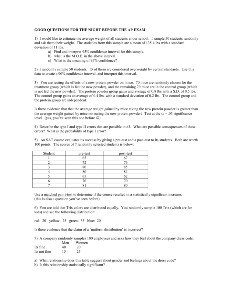
GOOD QUESTIONS FOR THE NIGHT BEFORE THE AP EXAM
1) I would like to estimate the average weight of all students at our school. I sample 50 students randomly
and ask them their weight. The statistics from this sample are a mean of 135.4 lbs with a standard
deviation of 11 lbs.
a) Find and interpret 95% confidence interval for this sample.
b) what is the M.O.E. in the above interval.
c) What is the meaning of 95% confidence?
2) I randomly sample 50 students. 15 of them are considered overweight by certain standards. Use this
data to create a 90% confidence interval, and interpret this interval.
3) You are testing the effects of a new protein powder on mice. 70 mice are randomly chosen for the
treatment group (which is fed the new powder), and the remaining 70 mice are in the control group (which
is not fed the new powder). The protein powder group gains and average of 0.8 lbs with a S.D. of 0.5 lbs.
The control group gains an average of 0.4 lbs. with a standard deviation of 0.2 lbs. The control group and
the protein group are independent.
Is there evidence that that the average weight gained by mice taking the new protein powder is greater than
the average weight gained by mice not eating the new protein powder? Test at the  = .05 significance
level. (yes, you’ve seen this one before )
4) Describe the type I and type II errors that are possible in #3. What are possible consequences of these
errors? What is the probability of type I error?
5) An SAT course evaluates its success by giving a pre-test and a post-test to its students. Both are worth
100 points. The scores of 7 randomly selected students is below:
Student
1
2
3
4
5
6
7
pre-test
65
72
80
80
65
70
81
post-test
67
76
85
84
62
70
80
Use a matched pair t-test to determine if the course resulted in a statistically significant increase.
(this is also a question you’ve seen before).
6) You are told that Trix colors are distributed equally. You randomly sample 100 Trix (which are for
kids) and see the following distribution:
red: 20 yellow: 25 green: 35 blue: 20
Is there evidence that the claim of a ‘uniform distribution’ is incorrect?
7) A company randomly samples 100 employees and asks how they feel about the company dress code.
Men
Women
Its fine
40
20
Its not fine
15
25
a) What relationship does this table suggest about gender and feelings about the dress code?
b) Is this relationship statistically significant?
8) Ideal proportions Once upon a time, a class like yours made measurements of their arm span and
height. There are 25 students in the class. They entered their results into a Minitab worksheet, requested
least squares regression of height based on arm span (both in inches) and obtained the following output:
Predictor
Constant
Arm span
s = 1.613
Coef
11.547
0.84042
Stdev
5.600
0.08091
R-sq = 87.1%
t-ratio
2.06
10.39
p
0.056
0.000
R-sq(adj) = 86.3%
a) Write the linear regression equation, defining all variables.
b) What is the slope of the line and what does it tell us?
c) What is the correlation coefficient and what does it tell us.
d) A student’s arm span was 60 inches and his height is 65 inches. Find the residual for this data point.
e)
Find a 95% confidence interval for the slope of the line.
9) A least squares regression line is given as:
a) log yˆ = 1.2x+2. Find the predicted value for x=2.
b) ln yˆ = 1.2x+2. Find the predicted value for x=2.
10) You are designing an experiment to test a drug that will decrease cholesterol levels. You will
randomly select 200 subjects. You will block by exercise level.
a) Describe the experiment completely.
b) What is double-blinding and how can it be used in this experiment?
11) 10 friends are all trying to reduce their cholesterol, and they ask to participate in the treatment group
together. Explain why this is a bad idea, using the term confounding variable.
12) Men’s heights are normally distributed with µ=69.5 and SD = 2.5.
Women’s heights are normally distributed with µ=65.5 and SD =2.5.
a) Find the probability that a randomly selected man is taller than 72 inches.
b) Find the probability that exactly 3 out of 5 mean are taller than 72 inches.
c) Find the probability that a randomly selected man and a randomly selected woman have combined
height over 140 inches.
d) Find the probability that a randomly selected woman is taller than a randomly selected man.
13) What is the outlier rule?
14) If p = .4, estimate p-hat from a sample size of 10 using these random digits:
13832 15623 98994 32398
KEY
1) First – check assumptions. 50 > 40 so sample size is large, so no checking of the data is necessary.
Random sample is stated. I will use a t interval because the standard deviation is from the sample.
Show mechanics:
X  z*
s
11
 135.4  2.021
n
50
Interval from TI-83 calculator (132.27, 138.53)
( Note t* comes from t-table, 95% , d.f = 49 (use 40). If you actually do the calculation, you’ll get a
slightly difference interval because the calculator will have t* for d.f.=49.)
I am 95% confidence that the true weight of all students in the school is in this interval.
b) 3.13
c)
This method will create an interval that captures the true population mean 95% of the time.
ˆ  50(.3)  15  10 and
2) I will perform a 1 proportion z interval. Checking conditions np
n(1  pˆ )  50(.7)  35  10 . Random sample is stated.
(note, we use a p-hat in an interval because there’s no hypothesized p to use)
mechanics are
pˆ (1  pˆ )
.3(.7)
 .3  1.645
n
50
pˆ  z *
(90% z* - can do invnorm (.95))
using ti-83 (.1934, .4066)
I am 90% confidence that the true proportion of overweight students is between 19.34% and 40.66%)
3)
Ho: µ1=µ2
Ha: µ1 > µ2
µ1 is average weight gain from mice on protein powder
µ2 is average weight gain from mice not on protein powder
Conditions:
Both samples are large: 70 > 40
Random selection of treatment and control group is stated
Assume independence
Perform 2 sample t-test
t=
X1 X 2
2
2
s1 s 2

n1 n 2

0.8  0.4
0.52 0.2 2

70
70
(use formula sheet to get this formula!)
using ti-83 calculator t = 6.214, p =7.7*10 -9, df = 90.5
Due to the extremely low p-value (less than the given alpha level of 0.05), we have evidence to reject the
null hypothesis. We have statistically significant evidence to believe that mice taking the protein powder
gain more weight).
4) Type I error is rejecting the Ho in error. So we reject the Ho, conclude that the protein powder works
and in reality, it does not cause a statistically significant difference in weight gain. (ie, we just got an
unusual sample that showed a difference). So then … the company makes a whole lot of this new protein
powder that really doesn’t work. Probability of this error is the significance level (5%) … note that’s the
probability before you even perform your experiment (ie, our low p-value in #3 indicates a lower chance
that a type I error occurred).
Type II error is accepting the Ho when you shouldn’t. So this is saying that the protein powder didn’t
work, when in reality it does (we just got an unusual sample again). A consequence is that you wouldn’t
produce the protein powder, when you really should have, it would have been a big seller.
Probability of type II error … really tough to calculate … you may want to review this (it was on a take
home quiz) if you have time.
5) a matched pair test is really a t-test on the differences. Calculate each difference and 1 var stat them …
I got mean =1.57 and Sd = 2.99. Use these numbers in a t-test
Ho: µdiff=0
Ha: µdiff>0
µdiff is average difference between pre and post test for pop of all students
Conditions: n is small, so look at and sketch a boxplot. No strong skew is seen, so continue. Random
selection of students is stated.
T-test on differences:
T=
X   1.57  0

s
2.99
n
7
on calc t=1.39
p=0.10 df=6
Due to high p-value, there is no evidence to reject the null hypothesis. Based on our sample, we have no
evidence that the course results in a statistically significant increase.
6) We’re looking at a chi-squared test of goodness of fit (the ti-83 doesn’t do this one)
Ho: dist of trix colors is uniform
Ha: dist of trix colors isn’t uniform.
(make sure you get specific with problem)
Conditions:
Expecteds are 25 of each color. 25 ≥10
Random sampling is stated.
2 
(obs  exp)2 (20  25) 2 (25  25) 2 (35  25) 2 (20  25) 2
=1+0+4+1 = 6




exp
25
25
25
25
d.f = categories -1=3
p= 
2
cdf (6,1000,3) =.111
due to the relatively high p-value, we do not have evidence to reject the Ho. There is no evidence that the
distribution of trix colors isn’t uniform.
7) a) it appears that women are more against the dress code than men are
b) To see if this relationship is statistically significant, we’ll perform a chi-squared test for independence.
Ho: no relationship between gender and dress code opinion
Ha: there is a relationship between gender and dress code opinion.
Conditions: all expected are ≥ 5
Expected matrix is
33 27
22 18
(this is matrix B after you perform test)
random is stated
Chi-squared test:
2 
(obs  exp)2 (40  33)2 (20  27) 2 (15  22) 2 (25  18) 2
=8.25




exp
33
27
22
18
p = 0.004 df =1 (2-1 times 2-1)
(note: numbers are from calc test)
Due to the very low p-value, we have evidence to reject the Ho of independence. Therefore, there is a
statistically significant relationship between gender and feelings about the dress code.
8) yˆ  .84042 x  11.547 x is the arm span and y is predicted height.
b) the slope of .84042 means that for every inch increase in arm span, an increase of .84 inches in height is
predicted.
c) r = .9332. (square root the r-squared). There is a strong positive linear correlation between arm span
and height.
d) y-hat = 61.97. 65-61.9722 = 3.0276
e) .84042  t *.08091  .84042  (2.069)(.08091) 2.069 is from the t-table, 95%, d.f.=n-2=23.
Final interval is (.673, 1.001) … We are 95% confident that the true increase in height for every inch
increase in arm span is in this interval.
9) plugging in, you get 4.4. But we are working with an equation that has undergone a log transformation.
Final answer is 10^4.4=25118.86
b) Same idea but its e^4.4=81.45
10) First, group all the high-level exercisers together and group the low level exercisers together. Within
each block:, first, number each subject. Then, using the random digit table, select half the block for the
treatment group. The remaining subjects will be in the control group and will not receive the drug ( a
placebo would be a good idea for this experiment so that the subject do not know whether they are in the
treatment or control group). After a designated period of time, compare the cholesterol levels of the
treatment group vs. the control group within both blocks.
A diagram:
New drug
High exercise
random
COMPARE
All subjects
Placebo
New drug
Low exercise
random
COMPARE
Placebo
b) double blinding means neither the evaluator nor the subjects know who is taking the drug vs. the
placebo. This is a good idea in this experiment… even though the evaluator is most likely using scientific
methods (checking blood) to measure cholesterol, by using double-blindness, it prevents any subconscious
or purposeful bias towards making our new drug work.
11) Since all 10 are going into the treatment group, and they are all trying to reduce their cholesterol,
confounding variables are introduced. If the treatment group shows an overall average decrease in
cholesterol level, it will be unclear if it is because of the drug or because 10 people in this group were
trying to reduce cholesterol before the experiment even started, and they may have improved their
exercise and eating habits, etc. resulting in cholesterol decrease.
Through blocking, we eliminate a known lurking variable of exercise. Through randomly choosing
treatment vs. placebo groups, we balance out any unknown lurking variables that may affect cholesterol
levels.
12) a) its normalcdf(72,100, 69.5,2.5) =15.87% (or by empirical rule, that’s 1 SD above the mean, and
answer is 16%).
Explain what calc button does! Or better if find z score of (72-69.5)/2.5 =1 and use table to get the 15.87%
b) 5C3 (.1587)3(.8413)2 = 0.028
c) Combined heights: mean = 135. SD = SQR(2.5 2+2.52)=3.53
normalcdf(140,1000,135,3.53) = .078. normalcdf find percentage of normal population above 140 given a
mean of 135 and SD of 3.53. (You could find the z-score and use table A as well.)
d) Difference is 4 inches. SD is again 3.53 inches (always add variances!).
Normalcdf(-1000,0,4,3.53) =.128

rubrics say lists of calc commands isn’t ‘work’. IF you can find z scores  z=(x-µ)/σ, that’s
probably enough work. Or at least explain that you know what calculator command is doing, that
may be fine as well (rubrics are unclear, sorry!)
13) Q3+(1.5*IQR) and Q1-(1.5*IQR). Anything outside of those boundaries are considered outliers.
14) Define 1-4 as yes, 5-9, 0 as no. You’ll only need the first 10 digits. You end up with 7 yes, a p-hat of
0.7.