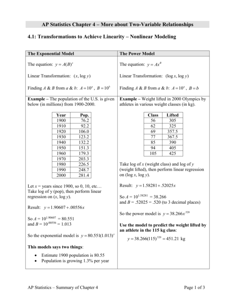
AP Statistics Chapter 4 – More about Two-Variable Relationships
4.1: Transformations to Achieve Linearity – Nonlinear Modeling
The Exponential Model
The Power Model
The equation: y  A( B) x
The equation: y  Ax B
Linear Transformation: ( x, log y )
Linear Transformation: (log x, log y)
Finding A & B from a & b: A  10a , B  10b
Finding A & B from a & b: A  10a , B  b
Example – The population of the U.S. is given
below (in millions) from 1900-2000.
Example – Weight lifted in 2000 Olympics by
athletes in various weight classes (in kg).
Year
1900
1910
1920
1930
1940
1950
1960
1970
1980
1990
2000
Pop.
76.2
92.2
106.0
123.2
132.2
151.3
179.3
203.3
226.5
248.7
281.4
Let x = years since 1900, so 0, 10, etc…
Take log of y (pop), then perform linear
regression on (x, log y).
Result: y  1.90607  .00556 x
Class
56
62
69
77
85
94
105
Lifted
305
325
357.5
367.5
390
405
425
Take log of x (weight class) and log of y
(weight lifted), then perform linear regression
on (log x, log y).
Result: y  1.58281  .52025 x
So A = 101.58281 = 38.266
and B = .52025 = .520 (to 3 decimal places)
So the power model is y  38.266 x.520
So A = 101.90607 = 80.551
and B = 10.00556 = 1.013
So the exponential model is y  80.551(1.013) x
Use the model to predict the weight lifted by
an athlete in the 115 kg class:
y  38.266(115).520  451.21 kg
This models says two things:


Estimate 1900 population is 80.55
Population is growing 1.3% per year
AP Statistics – Summary of Chapter 4
Page 1 of 3
4.2: Relationships between Categorical Variables
Two-Way Tables
A two-way table organizes counts from two categorical variables into rows and columns. They
are often used to summarize large amounts of data by grouping outcomes into categories.
Example: Below is data on a random selection of people who were categorized as having
low, moderate or high anger. Additionally, it was determined whether or not they had
coronary heart disease (CHD) at the end of a 4-year study.
CHD
No CHD
Total
Low anger
53
3057
3110
Moderate anger
110
4621
4731
High anger
27
606
633
Total
190
8284
8474
Marginal Distributions
The row totals and column totals give the marginal distributions of the two individual variables.
These numbers tell us nothing about the relationship between the two variables. They are simply
used to summarize the data.
Looking at the marginal distributions of anger rating in percents, we get:
Low anger
3110
 36.7%
8474
Moderate anger
4731
 55.8%
8474
High anger
633
 7.5%
8474
Note that this tells us what percent of the total fell into each of the three groups in the anger
rating variable. We see here that the majority of subjects were rated moderate, and a very
small percent were rated as high.
Conditional Distributions
To find the conditional distribution of the row variable, begin by focusing on a single column.
Then find each entry in the column as a percent of the column total. These percentages will tell
us about the association between the two variables in the table.
Now we look at whether anger tells has an association with CHD by calculating the percent
with CHD in each anger group.
Low anger
53
 1.7%
3110
Moderate anger
110
 2.3%
4731
High anger
27
 4.3%
633
We observe that the rate of CHD increases with anger level. So we conclude that the angrier you
are, the more likely you are to have coronary heart disease. The moral to this story is…chill out!
AP Statistics – Summary of Chapter 4
Page 2 of 3
4.3: Establishing Causation
The Question of Causation
An association between two variables doesn't necessarily mean that x causes y. Consider 3
possibilities in this situation and diagrams of the relationship between variables.
Causation – x does indeed
cause y
Common Response – a 3rd
variable, z, causes changes in
both x and y
Confounding – both x and a
3rd variable, z, cause changes
in y
In the above diagrams, z would be a lurking variable
Also consider that sometimes it is believed that x causes y, when it is actually the other way
around (y causes x). Call this Reverse Causation.
Confounding – definition
Two variables are said to be confounded when their effects on a response variable cannot be
distinguished from each other.
Examples
1. You observe that when more people wear coats there are also more people with colds.
Does wearing a coat cause the common cold? No – weather is a common response
lurking variable here. Cold weather causes more people to wear coats and more people to
get colds.
2. A study looks at the effects of after school tutoring and finds that students who get
tutoring fail classes at a higher rate than those who do not go to tutoring. So does tutoring
just cause students to do worse? No – this is reverse causation. Students go to tutoring
because they are doing poorly in class, not the other way around.
3. People who drink large amounts of alcohol tend to die earlier than those who do not.
Does alcohol cause an early death? Certainly, but other factors are to blame as well.
People who drink a lot probably also have other harmful behaviors such at poor diet,
which can also lead to early death. So both behaviors have causal links to early death, but
how much does each contribute? Hard to say, since these variables are confounded.
AP Statistics – Summary of Chapter 4
Page 3 of 3