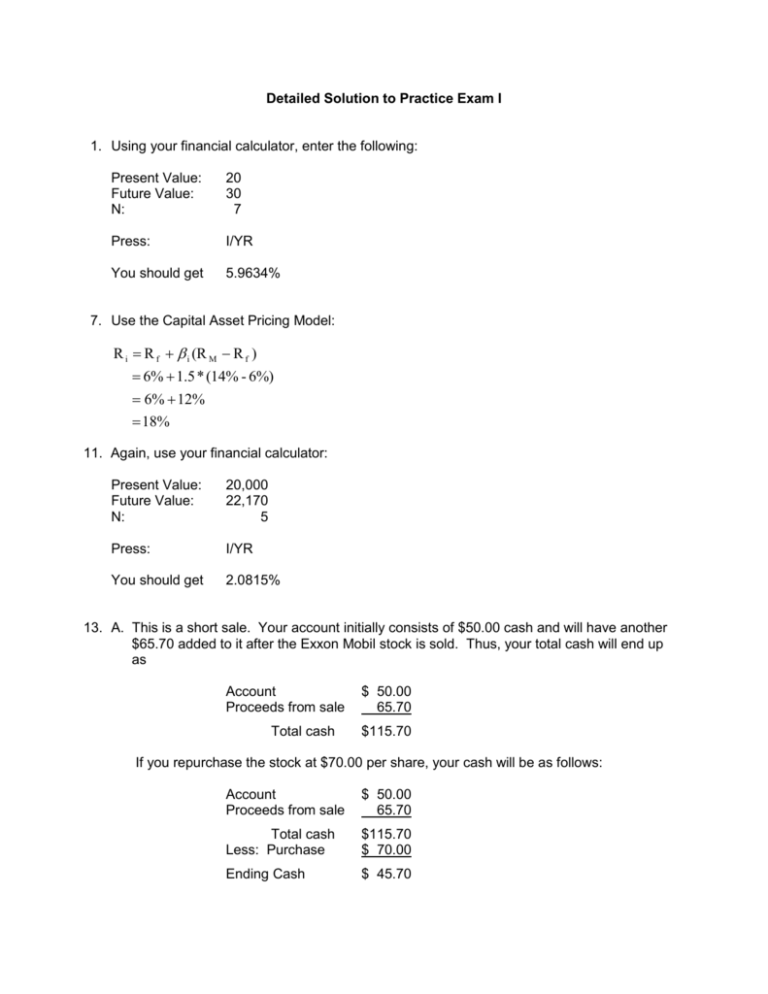
Detailed Solution to Practice Exam I
1. Using your financial calculator, enter the following:
Present Value:
Future Value:
N:
20
30
7
Press:
I/YR
You should get
5.9634%
7. Use the Capital Asset Pricing Model:
R i  R f   i (R M  R f )
 6%  1.5 * (14% - 6%)
 6%  12%
 18%
11. Again, use your financial calculator:
Present Value:
Future Value:
N:
20,000
22,170
5
Press:
I/YR
You should get
2.0815%
13. A. This is a short sale. Your account initially consists of $50.00 cash and will have another
$65.70 added to it after the Exxon Mobil stock is sold. Thus, your total cash will end up
as
Account
Proceeds from sale
Total cash
$ 50.00
65.70
$115.70
If you repurchase the stock at $70.00 per share, your cash will be as follows:
Account
Proceeds from sale
$ 50.00
65.70
Total cash
Less: Purchase
$115.70
$ 70.00
Ending Cash
$ 45.70
The $45.70 that you end up with is a loss of $4.30 per share on an equity investment of
$50.00 (the original account balance), or
(Ending Value - Beginning Value
Beginning Value
($45.70 - $50.00)

$50.00
$(4.30)

$50.00
 (8.6%)
Rate of Return 
B. Repeat the solution to Part A, but using a repurchase price of $55.00 per share.
Account
Proceeds from sale
$ 50.00
65.70
Total cash
Less: Purchase
$115.70
$ 55.00
Ending Cash
$ 60.70
The $60.70 that you end up with is a profit of $10.70 per share on an equity investment of
$50.00 (the original account balance), or
(Ending Value - Beginning Value
Beginning Value
($60.70 - $50.00)

$50.00
$10.70

$50.00
 21.4%
Rate of Return 
C. Use the equation for a short position margin that we had in Homework #1:
Margin 
Equity
Initial Price  Initial Equity - Current Price

Current Price
Current Price
$65.70  $50 - P
 0.3
P
or
$115.70 - P  0.3 * P
or
$115.70  1.3 * P
or
$89.00  P

14. A. To calculate the arithmetic average, just add up the returns and divide by the number of
periods of time:
Stock X
Stock Y
-10%
5%
12%
7%
10%
- 6%
4%
8%
4%
6%
24%
16%
Total
Average Return on Stock X 
24%
 4.8%
5
Average Return on Stock Y 
16%
 3.2%
5
B. The standard deviation formula for historic returns is the following:

(X i  X) 2
N -1
(X X  X) 2
X 
5 -1

(-0.1 - .048) 2  (0.05 - .048) 2  (0.12 - .048) 2  (0.07 - .048) 2  (0.1 - .048) 2
5 -1

(-0.148) 2  (0.002) 2  (0.072) 2  (0.022) 2  (0.052) 2
5 -1

(0.021904)  (0.000004)  (0.005184)  (0.000484)  (0.002704)
5 -1

0.03028
5 -1
 0.00757
 0.087 or 8.7%
Y 
(X Y  X) 2
5 -1

(-0.06 - .032) 2  (0.04 - .032) 2  (0.08 - .032) 2  (0.04 - .032) 2  (0.06 - .032) 2
5 -1

(-0.092) 2  (0.008) 2  (0.048) 2  (0.008) 2  (0.028) 2
5 -1

(0.008464)  (0.000064)  (0.002304)  (0.000064)  (0.000784)
5 -1

0.01168
5 -1
 0.00292
 0.054 or 5.4%
C. Stock X has a higher standard deviation so it is more risky.
D. The rate of return on a portfolio is a weighted average of the rates of return on the individual
assets:
RP  Ri * wi
i
 4.8% * .7  3.2% * .3
 3.36%  0.96%
 4.32%
E. Use the Capital Asset Pricing Model:
R X  R f   X (R M  R f )
 3%  0.5 * (9% - 3%)
 3%  3%
 6%
R Y  R f   Y (R M  R f )
 3%  0.75 * (9% - 3%)
 3%  4.5%
 7.5%